The 17th Asian-Australasian Association of Animal Production Societies Animal Science Congress
332
Estimating Consumer fs Response to Livestock Products Food Quality: Evidence
from Households in Indonesia
Mujtahidah Anggriani Ummul Muzayyanah, Suci Paramitasari Syahlani, Rini Widiati
Faculty of Animal Science, Universitas Gadjah Mada
Introduction
Consumer faces constraint on budget when they make consumption decision to maximize his/her utility. Allocating budget among commodity consumed is a must.
The economic variables, income and prices, and non-economic variable are the most important factors that determine food consumption. Cross-section household data provide household composition, expenditure, quantity consumed of food and nonfood, and other economic, social, and regional differences among households. As income increase, consumption of foods moves to higher quantity and quality food following their taste and preference change.
This paper attempts to study consumers’ response to quality in livestock products foods and estimates quality elasticity with respect to income over time
Methods
This study was used raw household data record from household expenditure data in urban and rural area of D.I Yogyakarta Province (here after DIY Province). The data used come from the detailed expenditure and consumption on food and non-food. The 2011 and 2013 Household Expenditure Survey (SUSENAS) was conducted by Central Bureau of Statistics (CBS) involving sampled-households.
Study of Hicks and Johnson (1968), Gale and Huang (2007) presented methodology to capture effect of quality through a nonlinear Engel relationship. According to their model, Engel curve expresses the relationship between household expenditure and income, as given in equation (1).
e(Y) = pq(Y) (1)
Deaton 1988 and Deaton 1997 noted that Engel’s curves using expenditure and quantity approach have always assume a log-linear function. But recent studies (Banks et al., 1997; Tey et al, 2009; Huang and Gale, 2009) have shown that a linear Engel curve cannot describe the real individual behavior.
Expenditure ej and quantity demanded qj of food items depends on economic and non-economic factor such as
household’s demographic variables z.
In this study, we define expenditure equation ej = f (y,z ) and quantity equation qj = f (y,z) using non-linear or
quadratic Engel relationship as
Ln q = α + β q (1/Y) + γqln Y + μ (2)
Similarly, for expenditure (e) and income (Y) relationship, equation (2) can be modified as:
Ln e = α + β e (1/Y) + γelnYy + μ (3)
Estimation of equations (2) and (3) would give values of parameters α , β , γ . If both β and γ are not equal to zero, then elasticities would be worked out, as follows:
η = - βq(1/Y) + γq (4)
ε = - βe(1/Y) + γe (5)
To analyse consumers’ response to quality over time, we modify equations (2) & (3), incorporating dummy-variable (D) for time differences, as follows.
Ln q = α1 + βq1(1/Y) + γq1lnY + α2D + βq2(D/y) + γq2ln(DY) + µ (6)
Ln e = α*1+ β*e1(1/Y) + γ*e1lnY + α* D + β*e2 (D/Y) + γ*e2ln(DY) + µ* (7)
Equations (6) & (7) incorporate dummy-variable (D = 0 for base period; D = 1 for new period) in both of its differential intercept.
Results and Discussion
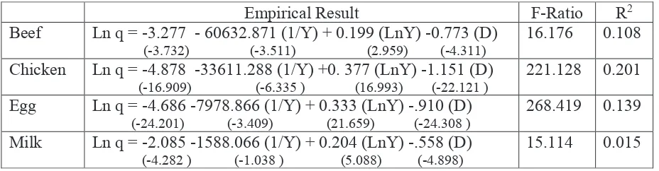
Using data of 7105 households from SUSENAS Household Survey data for DIY Province, conducted during 2011 and 2013, we estimated equations (6) and (7) for some livestock products. The results of the estimated equations along with diagnostic statistics (t-ratio, F statistic and R2) are provided in Table 1 (equation 6) and Table 2
The 17th Asian-Australasian Association of Animal Production Societies Animal Science Congress
333
(equation 7), and discussed and interpreted, as follows.
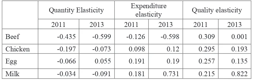
The differential intercept and differential slope, in both equations, have turned out to be statistically significant in these livestock products, indicating that significant changes have occurred in quantity and expenditure elasticities during 2013 compared to the base yearThe coefficients β q and β e, explained in equation (2) & (3), have turned out to be statistically significant in beef, chicken, egg and milk products, suggesting that log-log-inverse (LLI) formulation of the model validate the non-linear behavior of Engel curve for livestock products food in DIY Province. All selected livestock products foods appear to give similar results, with exception of milk (where β q is statistically insignificant) and egg (where β e is statistically insignificant).Quantity elasticity of demand for these livestock products with respect to consumer income is estimated for year 2011 and 2013 (Table 3). Expenditure elasticity with respect to income is estimated for 2011 and 2 The quality elasticity is thus positive and is estimated for 2001 and 2005.
Conclusions
The quantity and expenditure elasticities with respect to consumers’ income for livestock products foods have substantial changes during 2013 compared to base period of year 2011. The quality elasticity with respect to consumer’s income turns out to be positive for all livestock products foods. However, it declined in magnitude in almost all livestock products food except for milk products from year 2011 to 2013.
KEYWORD:livestock products foods, expenditure elasticity, quantity elasticity, quality elasticity, Indonesia
Table 1. Empirical Result of Quantity Model
Table 3. Quantity, Expenditure & Quality Elasticity (2011 and 2013)
Quantity Elasticity
Expenditure
elasticity
Quality elasticity
2011
2013
2011
2013
2011
2013
Beef
-0.435
-0.599
-0.126
-0.598
0.309
0.001
Chicken
-0.197
-0.073
0.098
0.12
0.295
0.193
Egg
-0.066
0.055
0.191
0.19
0.257
0.135
The 17th Asian-Australasian Association of Animal Production Societies Animal Science Congress
334
Table 1. Empirical Result of Quantity Model
Empirical Result
F-Ratio
R
2Beef
Ln q = -3.277 - 60632.871 (1/Y) + 0.199 (LnY) -0.773 (D)
(-3.732) (-3.511) (2.959) (-4.311)
16.176
0.108
Chicken Ln q = -4.878 -33611.288 (1/Y) +0. 377 (LnY) -1.151 (D)
(-16.909) (-6.335 ) (16.993) (-22.121 )
221.128 0.201
Egg
Ln q = -4.686 -7978.866 (1/Y) + 0.333 (LnY) -.910 (D)
(-24.201) (-3.409) (21.659) (-24.308 )
268.419 0.139
Milk
Ln q = -2.085 -1588.066 (1/Y) + 0.204 (LnY) -.558 (D)
(-4.282 ) (-1.038 ) (5.088) (-4.898)
15.114
0.015
(Figures in parenthesis represent t-ratios)
Table 2. Empirical Result of Expenditure Model
Empirical Result
F-Ratio
R
2Beef
Ln e = 6.927 - 62600.977 (1/Y) + 0.261 (LnY) - 0.561 (D)
(7.687) (-3.528 ) (3.773) (-3.041 )
39.173
0.228
Chicken
Ln e = 3.482 - 25914.287 (1/Y) + 0. 502 (LnY) - 1.214 (D)
(11.945) (-4.833 ) (22.386) (-23.085 )
365.436 0.294
Egg
Ln e = 3.370 -2936.291 (1/Y) + 0.446 (LnY) - 0.980 (D)
(18.561) (-1.338) (30.978) (-27.940)
546.566 0.248
Milk
Ln e =0.198 + 7337.349 (1/Y) + 0.772 (LnY) - 1.947 (D)
(0.566) (6.662) (26.739) (-23.709 )
269.610 0.213
(Figures in parenthesis represent t-ratios)
Table 3. Quantity, Expenditure & Quality Elasticity (2011 and 2013)
Quantity Elasticity
Expenditure
elasticity
Quality elasticity
2011
2013
2011
2013
2011
2013
Beef
-0.435
-0.599
-0.126
-0.598
0.309
0.001
Chicken
-0.197
-0.073
0.098
0.12
0.295
0.193
Egg
-0.066
0.055
0.191
0.19
0.257
0.135
Milk
-0.034
-0.091
0.181
0.731
0.215
0.822
REFERENCES
Bank, J., r. Blundell, a. Lewbell. 1997. Quadratic Engel Curves and Consumer Demand. The Review of Economics Statistics, 79: 527-539.
Deaton, A. 1998. Quality, Quantity and Spatial Variation of Price. American Economic Review, 78: 418-430. Deaton, A. 1997. The Analysis of Household Surveys: A Micro Econometric Approach to Development Policy.
Baltimore USA: John Hopkins University press
Gale, F. and K. Huang. (2007). Demand for Food Quantity and Quality in China. U.S. Department of Agriculture, Economic Research Service, ERR-32. Washington D.C.
Hicks, W. W. and S.R. Johnson (1968). Quantity and Quality Components for Income Elasticities of Demand for Food. American Journal of Agricultural Economics 50:1512-1517.
Huang, K.S, and F. Gale. 2009. Food Demand in China: Income, Quality, and Nutrient Effects. China Agricultural Economic Review, 1: 395-409.
Tey, T. S., S. Madnasir, M. Zainalabidin, S. Jinap, R. A. Gariff, 2009. Demand for Quality Vegetables in Malaysia”.