DOI 10.1007/s10640-009-9271-y
Optimal Timing of Climate Change Policy: Interaction
Between Carbon Taxes and Innovation Externalities
Reyer Gerlagh · Snorre Kverndokk · Knut Einar Rosendahl
Received: 28 January 2009 / Accepted: 10 February 2009 / Published online: 28 February 2009 © Springer Science+Business Media B.V. 2009
Abstract This paper addresses the impact of endogenous technology through research and development (R&D) on the timing of climate change policy. We develop a model with a stock pollutant (carbon dioxide) and abatement technological change through R&D, and we use the model to study the interaction between carbon taxes and innovation externalities. Our analysis shows that the timing of optimal emission reduction policy strongly depends on the set of policy instruments available. When climate-specific R&D targeting instruments are available, policy has to use these to step up early innovation. When these instruments are not available, policy has to steer innovation through creating demand for emission saving technologies. That is, carbon taxes should be high compared to the Pigouvian levels when the abatement industry is developing. Finally, we calibrate the model in order to explore the magnitude of the theoretical findings within the context of climate change policy.
Keywords Climate change·Environmental policy·Technological change·
Research and development
JEL Classification H21·O30·Q42
R. Gerlagh (
B
)Economics, School of Social Sciences, University of Manchester, Oxford Road, Manchester M13 9PL, UK
e-mail: [email protected] R. Gerlagh
Institute for Environmental Studies, Vrije Universiteit, Amsterdam, Netherlands S. Kverndokk
Ragnar Frisch Centre for Economic Research, Oslo, Norway K. E. Rosendahl
1 Introduction
In the coming decades radical policy interventions are necessary to bring a halt to the contin-uing increase in the atmospheric greenhouse gas concentrations when the aim is to prevent a potentially dangerous anthropogenic interference with the global climate system, see, e.g.,
IPCC(2007) andStern Review(2007). Though most scientists agree on the need for some abatement in the coming decades, there is a debate on whether the major share of these efforts should be pursued from the beginning, or whether the largest share of abatement efforts should be delayed to the future. Three reasons stand out among advocates of delayed action. First, due to the discounting of future costs, saving our abatement efforts for the future will allow us to increase our efforts considerably at the same net present costs. Second, delaying emission reduction efforts will allow us to emit larger cumulative amounts of greenhouse gases, and thus to abate less in total, due to the natural depreciations of the atmospheric greenhouse gas concentrations. Third, delaying abatement efforts will allow us to benefit from cheaper abatement options that are available in the future, and also to develop these options through innovation. The first two arguments have taken firm root in the literature, thanks to—among others—the analysis byWigley et al.(1996).1 The third argument, however, based on pre-sumed technological advancements in abatement options, has raised a lively debate among economists studying technological change in relation to climate change, and more generally, environmental policy.
There are arguments for accelerating abatement efforts rather than delaying them. Energy system analyses have clear empirical evidence for so-called experience curves suggesting that new low-carbon energy technologies, which will define the major long-term options for carbon dioxide emission reduction, need to accumulate experience for costs to come down sufficiently to make these technologies competitive.2Based on these experience curves, the more general argument is made that there is a need for up-front investment in abatement tech-nologies to make them available at low prices, and thus, technological change would warrant early abatement action rather than a delay (Ha-Duong et al. 1997;Grübler and Messner 1998;van der Zwaan et al. 2002;Kverndokk and Rosendahl 2007). Models exploring the experience curves are typically referred to as learning by doing (LbD) models.3Many energy system models add another reason for a smooth transition towards clean energy supply, which is that diffusion of new technologies need the turnover of all existing vintages and therefore takes a considerable time (Knapp 1999). A too rapid switch of the capital stock towards an entirely new technology is considered unrealistic (Gerlagh and van der Zwaan 2004;Rivers and Jaccard 2006).
Objections have been raised to these arguments. Though experience and diffusion curves have a strong empirical basis, many economists consider it a mechanistic view on technolog-ical development hiding the incentive-based structures that determine the level of research efforts by innovators. They prefer models with an explicit treatment of research and devel-opment (R&D) as the engine of innovation, and they have found that modelling innovations through R&D can lead to potentially very different outcomes on optimal timing of abatement policy. An important difference between LbD and R&D models is that the latter category of models does not assume from the outset that the technology needs to be used for its costs
1They used these arguments to make the case that emission paths developed by theIPCC(1995) for ceiling atmospheric carbon dioxide concentrations tended to put too much effort up-front, while a delayed abatement response would be more cost-efficient.
2SeeLieberman(1984) for an early contribution focused on the chemical industry, andIsoard and Soria (2001) for a recent empirical analysis for energy technologies.
to fall. Thus, through R&D, future cheap abatement options may be made available without the need to use these abatement options while costs are still high. In an R&D model, it is then most efficient to focus mainly on R&D in the early stages of abatement policy, without employing the technologies, and to apply them only after the costs have sufficiently come down. Indeed,Goulder and Mathai(2000) found this pattern as an optimal environmental policy and they concluded that whereas LbD may warrant an advance of using abatement technologies compared to a situation without technological change, the presence of R&D unambiguously implies a delay in the use of such technologies.
The first objective of this paper is to extend the discussion on the timing of abatement to include the timing of climate change instruments. That is, we will not only ask the question as to whether the possibility of R&D implies a delay or advance of abatement, but rather, we will ask whether optimal carbon taxes are ahead of or delayed with respect to Pigouvian taxes and whether research subsidies should be constant, decreasing or increasing over time. This is the first research question.
Second, we will extend the analysis of optimal climate change policy with R&D to a second-best context, i.e., when we have several imperfections, but insufficient policy instru-ments available to correct them all. Caution is needed when results—such as the delay in optimal abatement thanks to R&D—depend on first-best assumptions, since such a first-best innovation-abatement solution can be reached only when policy makers have a rich instru-ment set available. R&D market imperfections may be different for climate change specific technologies such as, say, energy saving innovation and non-carbon emitting energy sources, compared to other technologies. In that case, policy makers need to have an instrument avail-able tailored to climate change-related R&D to bring emission reduction R&D efforts to their socially optimal level. However, while innovation subsidies certainly exist, it is hard for a government to commit to subsidise all new innovations that create positive spillovers, as well as to identify these spillovers, see, e.g., the discussion inKverndokk et al.(2004).
Gerlagh et al.(2008) also show that with a finite patent lifetime, optimal innovation policy depends on the stage of the environmental problem, which may also be uncertain to the pol-icy makers. In the absence of such tailored climate-change R&D instruments, polpol-icy makers may use a common R&D instrument such as R&D subsidies over all sectors, and a generic climate change instrument such as carbon taxes or emission permit markets to target climate change goals. Since energy related R&D makes up only a small portion of economy-wide R&D expenditures, we consider it a natural assumption that R&D subsidies are exogenous to the climate change policy problem, and consequently, the policy maker has to rely on one instrument, say the carbon tax, to steer both abatement levels and climate change-specific R&D efforts. Since now the carbon tax affects both abatement efforts and innovation, the functioning of the innovation market within the energy sector, i.e., how the gap between private and social returns on R&D develops, becomes of crucial importance for determining the efficient level of the carbon tax. The second research question is thus how the optimal carbon tax should develop, relative to the Pigouvian tax, in a second-best setting.
For our study we develop an R&D model in line with the endogenous growth literature and assume that R&D efforts are based on market-based incentives through patents. Patents have different welfare implications. They give an incentive for innovation as they protect the holders from others directly using their innovation in production, but they also create a static inefficiency as patents allow monopolistic supply by the patent holder. A long patent lifetime increases the incentives for innovation but increases the static inefficiency.4At the same time,
patents disclose the knowledge base underlying the innovation, which then can be used by rivals to develop substitute technologies. These properties can lead to intricate connections between R&D dynamics and climate change policy (cf.Encaoua and Ulph 2004), and we need to see how they alter the first-best timing results.
We expect that an R&D model may present similar results as the LbD models when we study innovation in a second-best R&D setting with finite lifetime of patents. Whereas in a first-best R&D model with an infinite patent lifetime, it is possible that innovators develop new technologies and continually improve these without them to be used in production, in a second-best R&D model with finite patent lifetime, innovations will only occur when they are used in production before the patent’s expiration date. This mechanism is similar to the mechanism in LbD models, where technology only advances if it is used. Thus, the represen-tation of finite lifetime of patents in an R&D model will lead to the required use of abatement technologies in earlier periods to guarantee that innovators can earn back the costs of R&D. The argument above makes clear that a finite patent lifetime creates an appropriation problem for innovators who cannot fully capture the social value of their innovations in the long future. Many R&D models incorporate the idea that innovators cannot appropriate the full value of their innovations—Nordhaus(2002),Popp(2004) andGerlagh and Lise(2005) make precise assumptions on this. But whereas in the broad innovation literature the finite lifetime of patents is a common reason for this feature (for an early contribution, seeNordhaus 1969), in the environmental economics literature, the time dimension of the appropriation problem is mostly neglected. If the appropriation gap would be a constant fraction of the social value (as assumed in these models), then a constant innovation subsidy would be suffi-cient to correct for this market failure. If, however, patents expire, innovations will be biased towards technologies that pay back within the patent’s lifetime, while there is no incentive to develop and improve technologies whose value lies in the farther future. A generic R&D subsidy cannot correct for this timing dimension of the appropriation problem, and instead, a complementary climate policy may be required for its correction. We also refer toGerlagh et al.(2008) where we use a related model to the one presented below, but in continuous time, and without research subsidies but with the lifetime of the patent endogenously determined. This paper is organised in the following way. In Sect. 2 we develop a partial model for abatement, emissions and a greenhouse gas atmospheric stock. The model has discrete time steps, and technological change is driven by theRomer(1987) type of endogenous growth through increasing varieties, based on the ‘love of variety’ concept (Dixit and Stiglitz 1977). We analyse optimal climate change policies in Sect. 3, starting with a first-best setting as inHartman and Kwon(2005) andBramoulle and Olson(2005, cf Proposition 8). In the first best solution all policy instruments to correct for imperfections are available. Then we con-sider the second-best setting, where an R&D subsidy is not available, for which we analyse the development over time of efficient carbon taxes relative to Pigouvian taxes. In Sect. 4 we study the cost-effective policy, i.e., when there is a fixed restriction on the build up of the atmospheric concentration of greenhouse gases. As inHart(2008) andGreaker and Pade
(2008), our timing analysis specifically addresses transition paths where the abatement sector is small initially but rapidly increases in size, followed by a slower growth when the sector becomes mature. Different fromGoulder and Mathai(2000), the timing analysis is not based on a comparison of multiple scenarios, e.g., one with and another one without endogenous technological change.5Instead, we analyse the development over time of research subsidies and the gap between efficient carbon taxes and Pigouvian taxes in the first- and second-best
setting. The relative gap between the two taxes tells us something about the relative stringency of climate change policy compared to the social cost of pollution, and we are particularly interested in its development over time.
Our focus on the gap between efficient carbon and Pigouvian taxes puts our analysis in a broad strand of literature. Much of this literature focused on tax interaction effects (c.f.
Bovenberg and de Mooij 1994) and it raised lively debates in policy circles when it explored the potential for so-called double dividends. In addition to tax interaction, reasons for a divergence between efficient carbon and Pigouvian taxes include trade effects (Hoel 1996), scale effects in production (Liski 2002), and, more recently, the processes underlying tech-nological change.Rosendahl(2004) shows that in an LbD model, the carbon tax should be higher than a Pigouvian tax, with the largest gap for those countries and sectors that gen-erate most of the learning. In a similar fashion,Golombek and Hoel(2005, Proposition 9) show that in a climate change treaty the optimal carbon price can exceed the Pigouvian level when abatement targets lead to innovation and international technology spillovers that are not internalised in domestic policies.6Our paper studies the dynamics of this gap between efficient and Pigouvian carbon taxes, in relation to endogenous technological change.
Finally, in Sect. 5 we carry out some numerical calculations to further investigate the substance of the theoretical findings. Throughout the simulations, the model parameters are chosen to reflect the common climate change context. Sect. 6 concludes.
2 Model Set Up
We consider an economy where there are concerns for the environment due to stock pollution. The set up of the model is general, but the interpretation of the pollutant will be in terms of carbon dioxide emissions following from the combustion of fossil fuels. More generally, we assume a benchmark emission path and a demand for abatement of emissions because of environmental considerations.
2.1 The Abatement Sector
The model of research and development (R&D) is based on Romer’s endogenous growth model (Romer 1987,1990;Barro and Sala-i-Martin 1995). The model has an infinite horizon with discrete time steps,t=1, . . .,∞. There is one representative abatement sector, which could either be interpreted as an alternative, emission-free resource sector (e.g., renewables) or as abatement of emissions (e.g., fossil fuels supplemented with carbon capturing and storage). There are Ht producers of abatement equipment at each point of timet, and an
R&D sector producing new ideas or innovations. Technological progress takes the form of expansion in the number of abatement equipment varieties. The producers of the abatement equipment own patents and, therefore, receive monopoly profits. However, they have to buy the innovations from the R&D sector, where innovators are competitive and use research effort as an input. We assume that patents last for one period, and so innovations are public
Footnote 5 continued
comparison between the two scenarios is mainly driven by the difference in technology paths, and is largely independent of the source of technological change, be it endogenous or exogenous. Though our set up is not directly comparable withGoulder and Mathai(2000), our broader context is comparable as both study the timing of action.
goods thereafter. Hence, there are positive spillovers to innovation from the previous-period stock of innovations (standing on shoulders). Also, we assume negative externalities from aggregate current research through fishing out of ideas. Thus, in this model there are three imperfections related to innovations; too little production of abatement equipment due to monopolistic competition, positive spillovers of the earlier period innovation stock on new innovations, and negative spillovers of total research effort on new innovations. Thus, the market outcome of innovations may exceed or fall short of the social optimal level.
LetEbe emissions of the stock pollutant,Yis benchmark emissions without any climate change policies, whileAis abatement. Thus, total emissions are as follows:7
Et =Yt−At (1)
Production of abatement requires intermediate flow inputs Zt, and the use of abatement
equipmentxi for various varietiesiǫ[0,Ht]whereHt is the number of equipment varieties.
Htcan be interpreted as the state of knowledge.8
At= B Ztα a strict inequality implies that there is a fixed factor in production, e.g., due to site scarcity for renewables. The presence of a fixed factor implies that the value of output is strictly larger than the value of all variable inputs. In that case we can specifyBasB=c F1−α−βγ, where
Fis the fixed factor andcis a constant, such that the total value of output is fully attributed to all inputsZ,xi, andF.9
The different abatement equipments are neither direct substitutes nor direct complements to other specific equipments. That is, the marginal product of each abatement equipment is independent of the quantity of any particular equipment, but depends on the total input of all other equipment varieties together. Since all varieties have the same production costs and decreasing marginal product, in equilibrium the same quantity will be employed of each equipment. Thus, assuming that the equipment can be measured in a common physical unit, we can write xi = X/H, where X is the aggregate input of abatement equipment. The
production identity then becomes:
It is clear that while the abatement sector has (short-run) decreasing returns to scale for given technologyHt,α+βγ ≤1, there are possibly long-run increasing returns to scale when
7The relation between emissions and benchmark emissions is specified as a linear function for convenience of notation. A more general function would give the same qualitative results. In the numerical simulations in Sect. 5, we use a CES aggregation.
8Note that the productivity of abatement equipment does not diminish over time. This means that the benefit from a new innovation on abatement production is higher at the earlier stage of abatement as it contributes to the knowledge base for a longer period. This would be an argument for a longer lifetime of patents at the early stage of emission abatement, seeGerlagh et al.(2008). See also the discussion in Sect. 3 below on the optimal R&D subsidy.
α+γ >1, due to the endogenous nature of technologyH.10Now consider the case where abatement efforts have to increase over time continually to maintain a ceiling on the atmo-spheric stock of greenhouse gases jointly with an increasing overall economic activity. For
α+γ <1, the abatement expenditures will have to increase more than proportionally with the abatement effort. Forα+γ =1, the costs of abatement rise in proportion with abatement levels. Forα+γ >1, the price of abatement decreases, and total expenditures increase less then the abatement effort.
Assume now that the public agent implements a carbon taxτt, or more generally an
envi-ronmental policy that induces a market cost of emission,τt. From (1) we see that this translates
into a market price for abatementAt. The abatement producer’s optimisation problem is:
MaxτtAt−Zt−
Thus, the abatement producer maximises the value of abatement minus the abatement costs. The first order conditions of this maximisation problem determine the abatement pro-ducer’s demand forZandxi:
From (5) we see that the costs ofZshould equal the shareαof the production value, where
αexpresses the relative contribution ofZin production.
The demand forxt,iis given by (6). Alternatively, by rearranging (6) we can also express
the demand for aggregated input of abatement equipment usingxi =X/H,andpt,i= pt:
ptXt=βγ τtAt. (7)
Thus, the demand for abatement equipment is falling in the own price, but increasing in the carbon price.
2.2 Production of Abatement Equipment
The producers of abatement equipment own patents and therefore act as monopolists. Their costs of producing intermediatesxt,iare set to unity, and they maximise profits (or the value
of the patent),πt,i,taking into account the falling demand curves for abatement equipment.
For a patent valid for one period, we get the following maximisation problem:
Maxπt,i=xt,i
pt,i−1
, (8)
10An interesting case arises whenγ =1–α. There are decreasing returns to scale for a given technological levelHt, e.g., due to a fixed factor. This can be understood as the short-term feature of the model. At the same
subject to (6).
The first order condition from maximising (8) with respect topt,idetermines the price of
the abatement equipment:
pt,i= p=1/β. (9)
From (7) and (9) we find the market equilibrium forX:
Xt =β2γ τtAt. (10)
As all varieties are identical (xi = X/H), and prices are equal across varieties, see (9), the
value of a patent is also equal for all innovations, i.e.,πt,i=πt. Using this in addition to (8),
(9), (10) andxi= X/H, we find the value of all patents:
πtHt=(1−β) βγ τtAt. (11)
2.3 The Innovation Process
The producers of abatement equipment buy patents from innovators that operate in a com-petitive market.11Innovators develop new varieties according to the following production function:
ht,j=rt,j(Ht−1/Rt)1−ψ, (12)
wherert,j is the research effort of innovator j,ht,j is the number of varieties produced by
this innovator, and we assume 0< ψ < 1.Rt denotes aggregated research efforts by all
innovators.
As seen from the production function in (12), there is a positive externality through a spillover from the previous period knowledge stock throughHt−1, and a negative externality
through fishing out of ideas, through current researchRt.12The former is typically referred
to as ‘standing on the shoulders’. The latter mechanism captures the idea that when the num-ber of researchers increases, more researchers will find the same new variety that is just on the frontier of current knowledge, but only one of the discoverers will be able to patent the new variety. Thus, for every researcher, the aggregate research effort enters negatively in his innovation production function. We also see that both externalities are higher the lower the value ofψ.
The innovators maximise profit with respect to research effort, where the price of the innovation equals the monopoly profit of equipment producers, or equivalently the value of the patent.
Maxπtht,j−rt,j, (13)
subject to (12).
11Alternatively we could assume that the innovators are producing the abatement equipments, such that they own the patents and get the monopoly rent. This would not change the arguments or conclusions of the analysis. 12Encaoua and Ulph(2004) distinguish between knowledge and technology information flows.Knowledge
flowor knowledge diffusion is equal toςHt−1, which means that a fraction 0< ς <1 of previous knowledge is public information at timet. Thetechnology flowis the technology spillover according to which a technology can be imitated by others, such that a patent does not offer a perfect protection to its holder. In our model this would mean thatχHtwill be private property of the patent holders, where 0< χ <1, while (1−χ)Htcan
The price of research effort is set equal to one. First order conditions give that the unit cost of research (i.e., one) is equal to the value of the patent,π, multiplied by the productivity ofr.
Due to the zero-profit condition, in equilibrium the value of all patents is equal to the value of all research effort:
πtHt=Rt. (14)
Substitution of (14) in (11) and aggregation of (12) give the following two conditions for research effort and knowledge dynamics in the economy:
Rt =(1−β) βγ τtAt (15)
Ht = Rψt H
1−ψ
t−1 . (16)
For any given carbon price policy pathτt, the five equations (3), (5), (10), (15) and (16)
define a market equilibrium through the variablesAt,Zt,Xt,Rt,Ht.13
3 Efficient Policy Implementations 3.1 First-Best Policy
The social planner aims at minimising the present value of abatement costs plus the dam-age from the stock pollutant. This can for instance be interpreted as the damdam-age from the concentration of carbon in the atmosphere, i.e., the carbon stock. The minimisation problem becomes (whereδ< 1 is the social discount factor):
Min
∞
1
δt−1[Zt+Rt+Xt+D(St)], (17)
subject to (1), (3), (16) and stock accumulation dynamics
St =(1−ε)St−1+Et. (18)
The social abatement costs are the sum of the costs ofZ,RandX, which all have unit cost equal to 1.
D(S)is the damage cost function, where damage depends on the stock of emissions,S. We assume thatD(S0)≥0,D′(St) >0 andD′′(St) >0, and that the stock depreciates
by the rateε <1.
The first order conditions from this minimisation problem are:
Zt =αθtAt (19)
Xt =βγ θtAt (20)
Rt =ψ ηtHt (21)
ηtHt =δ (1−ψ ) ηt+1Ht+1+(1−β) γ θtAt (22)
θt = D′(St)+δ (1−ε) θt+1. (23)
Note thatθt −λt ≥0, whereλt is the dual variable for Eq.1, and, hence, the current
value shadow price of emissions.θt is often referred to as the Pigouvian tax. Note also that
13Strictly speaking, uniqueness of the equilibrium requires decreasing returns to scale within one period, that
θt is equal to the social price (or marginal value) of abatement in this model, asEt andAt
are perfect substitutes, and since At has no effects on knowledge (as it would in an LbD
model).ηt ≥0 is the dual variable of Eq.16and, therefore, the current value shadow price
of knowledge.
The first order conditions forZandXdefined by (19) and (20), are similar to the corre-sponding conditions for the market equilibrium given by (5) and (7), with the exception that market prices are replaced by the corresponding social prices.
As seen from (21), the value of research should equal the shareψ of the social value of knowledge.ψ expresses the relative contribution ofRin producing knowledge. Eq.22
shows that the shadow price of knowledge is in general positive, but equal to 0 if there is no abatement throughout the time horizon.
According to (23), the social cost of emissions at timet,θt, is the present value of the
damages caused by one unit of emission emitted at timet. It follows from a comparison of (5) and (19) that in the first-best policy,θt is equal to the optimal emission taxτt at timet.
As there are three types of imperfections in the model; pollution, imperfect competition in the market for abatement equipment, and positive and negative externalities of research effort, we would need three policy instruments to implement the social optimum: an emission tax,τt, a subsidy on abatement equipment,sx,t, and a subsidy/tax on research,sr,t. We can
then write the market conditions corresponding to (19), (20) and (21) as
Zt =ατtAt (24)
First, Eq.24is equal to the market condition defined in (5). Second, replacingptin Eq.7with
(1−sx,t)pt, gives the demand forXtexpressed by (25). Finally, (26) is derived in the same
way as Eq.11and15, apart from that we use (25) instead of Eq. (10). The price innovators pay forrt is now set to (1−sr,t) instead of unity.
Setting the carbon price equal to the Pigouvian tax, i.e.,τt =θt, implements the optimal
use ofZt, see (19) and (24). To find the optimal subsidy rate on abatement equipment,sx,t,
Inserting the first-best level ofRfrom (21) gives after some calculation:
sr,t =1−(1−β) γ θtAt/ψ ηtHt. (29)
The optimal level ofsr,t in Eq.29 may be positive or negative. This is because research
effort has both positive and negative external effects. The positive external effect is that cur-rent research contributes to future research, and this use of knowledge is not protected. The negative externality is the fishing out described below Eq.12.
The development of the research subsidy/tax,sr,t,will depend on the development of the
ratioθtAt/ηtHt, i.e., the social value of abatement relative to the social value of knowledge,
time, it is useful to define the abatement expenditure growth factor asφt =τt+1At+1/τtAt. In
a mature abatement sector, this growth factor is constant. For an infant industry, growth will exceed the matured growth level. When the sector is becoming mature, expenditure growth will gradually fall from its infant level to its mature level. We define the abatement sector to be
maturingwhenφt ≥φt+1for allt≥0. We can now answer the first research question: how does the possibility of technological improvement through R&D affect the timing of climate change instruments? The answer is that, where R&D may delay the abatement level as shown inGoulder and Mathai(2000), at the same time it requires the advance of the climate-change related research subsidies. That is, research subsidies will have to start at a high level and fall over time. Note that this is related to our assumption that the productivity of abatement equipment does not diminish over time. Thus, the benefit from a new innovation is higher at the earlier stage of emission abatement as it contributes to the knowledge base for a longer period. The following proposition answers our first research question.
Proposition 1 Through a tax on emissions equal to the Pigouvian tax,τt = θt, a subsidy
on abatement equipment equal to sx,t =1−β, and a subsidy/tax on R&D effort equal to
sr,t=1−(1−β)γ θtAt/ψ ηtHt, the first best outcome can be implemented. For a maturing
abatement sector, the efficient R&D subsidy/tax sr,twill fall over time.
Proof The first part of the proposition has been shown above. To prove that the R&D subsidy will fall over time, we consider (29) and see that it suffices to prove thatηtHt/τtAtdecreases
over time. Notice thatθt =τt. Writing out Eq.22for the entire horizon, we have
ηtHt/θtAt=(1−β)γ{1+δ(1−ψ )φt+ [δ(1−ψ )]2φtφt+1+ · · ·}. (30)
It is obvious that whenφtis decreasing int, then when we compare the equation forηtHt/θtAt
andηt+1Ht+1/θt+1At+1, in the latter equation, each of the terms on the right-hand side will
be smaller, and thus,ηt+1Ht+1/θt+1At+1≤ηtHt/θtAt. ⊓⊔
3.2 Second-Best Policy
Even if the social optimum in principle may be implemented using the appropriate number of policy instruments, it may be hard to target R&D at the firm level (as long as R&D effort is not completely undertaken in the public sector). For instance, R&D is not specified as a separate activity or sector in most national accounts. Consequently, it is difficult to use instruments such as a subsidy to producers of abatement equipment and a subsidy/tax on research effort. Based on this, we specify a second-best optimum, where the social planner has only one policy instrument available, namely the carbon price.
The second-best optimisation problem of the social planner is, therefore, the minimisation problem (17) subject to (1), (3), (16), and (18), but also subject to the market equilibrium for Z, Rand X given by Eqs.5,10and15. The social planner now sets the value of τt
that minimises social costs subject to the functioning of the atmospheric carbon stock, the technology stock, and the different markets.
We can solve this social optimisation problem by substitution. In combination with (5), Eqs.10and15give
Xt =
β2γ /αZt (31)
Substitution of (31) and (32) in (17), (3), and (16) give
Letηtbe the dual variable for Eq.35. The first order condition forZt and the optimal level
ofHtare given by
wZt =(α+βγ )θtAt+ψηtHt (36)
ηtHt =δ(1−ψ )ηt+1Ht+1+(1−β)γ θtAt. (37)
In addition, Eq.23carries over from the first-best solution. While Eq.37is equal to the cor-responding equation (22) in the first-best solution, the first order condition forZis different due to the restrictions on the use of policy instruments (compare (36) with (19)).
From (5) and (36) and inserting forw, we derive
τt/θt =1+
ψ/ (α+ βγ )ηtHt/θtAt (38)
This formula calculates the efficient second-best carbon price relative to the Pigouvian tax on basis of the constant parametersα,β,γ,ψand the ratio of the value of knowledge over the value of abatement,ηtHt/θtAt. As we see from (38),τt/θt >1, which means that the
efficient carbon price will be higher than the Pigouvian tax. Notice that this result also holds when there are decreasing returns to scale,α+γ <1. The main mechanism leading to higher carbon taxes, compared to the Pigouvian level, is the monopolistic undersupply of abatement equipment.
Willτt/θtrise or fall over time? As seen from (38), this depends on the development in the
ratio of the value of knowledge over the value of abatement, i.e.,ηtHt/θtAt. This means that
the development inτt/θtfollows a similar path as the development in the optimal subsidy/tax
on research, see (29). Thus, without the possibility to target research effort, the difference between the efficient emission tax and the Pigouvian tax should mimic the development in the optimal research subsidy/tax. This answers the second research question. In the second best setting with constant R&D subsidies, the carbon tax should be accelerated compared to the Pigouvian tax.
Proposition 2 In the second-best model, the efficient carbon price,τt, will always be higher
than the Pigouvian tax,θt, as long as abatement is positive. For a maturing abatement sector,
the relative difference between the efficient carbon price,τt, and the Pigouvian tax,θt, will
fall over time.
Proof From (5) and (36), we calculate a slight deviation from (38),
θt/τt=1−
ψ/(α + βγ )[ηtHt/τtAt], (39)
which is less then unity. It suffices to prove thatηtHt/τtAt decreases over time, which
4 Cost Effective Policy
When pollutant damagesD(S)are highly uncertain, such as damages from global warming, an alternative policy might be to minimize the costs associated with a constraint on the build up of the pollutant, set by a ceiling, S¯. Such a cost-effective policy is likely to induce a
high growth in abatement expenditures before the ceiling is hit. The minimisation problem becomes:
Min
∞
1
δt−1[Zt+Rt+Xt], (40)
subject to (1), (3), (16), (18) and the stock restrictionSt≤ ¯S. We maintain the first order
conditions (19), (20), (21), and (22), but (23) becomes
θt=δ (1−ε) θt+1+µt, (41)
whereµt is the dual variable of the constraintSt ≤ ¯S. If the pollutant stock starts at very
low level,St << S¯, the social marginal costsθt grow at a factor 1/δ(1−ε). After the
pollution stock ceiling is reached, the social marginal costs grow at a lower rate. Unless the initial knowledge stock is very high, this pattern forθtof a high growth rate followed by a
levelling off (but not necessarily a continuous drop after the ceiling is reached) will result in a similar pattern for abatement levelsAtand knowledge levelsHt. The formal establishment
of such a pattern is very tedious as the growth path for all variables depends on the initial knowledge stock. An obvious assumption would be to require that the economy starts at a balanced growth path, but one cannot assume such. For example, when the abatement sector has overall increasing returns to scale:α+γ >1, one can show that prices cannot go up on a balanced growth path with increasing abatement effort. Thus, the economy may not start at a balanced growth path, and we allow ourselves a relatively loose statement in the next proposition to describe the feature that abatement expenditures grow rapidly before the ceiling is hit, and grow less rapidly thereafter, but the growth rate of expendituresφtmay not
necessarily decrease monotonically.
Proposition 3 Until the ceiling is reached, assume that the abatement sector is maturing and the growth in expenditures exceeds the growth at any time after the ceiling is reached. Then, in a first-best allocation, the cost-effective R&D subsidy/tax stwill fall over time until the
ceiling is reached. Similarly, in the second-best R&D model, the relative difference between the efficient carbon price,τt, and the Pigouvian tax,θt, will fall over time until the ceiling is
reached.
Proof The proof is very similar to that of Proposition 1. LetT be the time that the ceiling is reached, the assumption states thatφt > φv > φwfor allt < v <T < w. It is now easy
to see that in Eq.30, when we move fromt <T tot+1, in each element at the RHS we replaceφt by someφvorφw, and thus the RHS must drop. The same argument applies to
the second-best model. ⊓⊔
5 Simulations
In this section we want to supplement the theoretical findings by developing and simulating a numerical model that mimics a transition from a fossil fuel based to a carbon free energy system. The speed of transition is determined by technological progress, driven by policies and market forces. In particular, the numerical model gives insight into the magnitude and development over time of the relationship between the optimal carbon price and the Pigouvian tax in a situation where it is not possible to specifically subsidize abatement cost reducing research.
5.1 Calibration
We set out to calibrate a model that reproduces key characteristics of the climate change debate in a stylised manner. The model is consistent with the theoretical model set up in Sect. 2, except for Eq.1. In the analytical model, it was assumed that abatement is a purely additional activity, decreasing emissions one-to-one. The assumption in the analytical model is convenient and common practice in theoretic models, but in the context of climate change policy, abatement may better be treated as the substitution of non-carbon energy sources for fossil fuels, and rather than assuming perfect substitution between the two, we assume a CES-aggregate of energy production.14Equation1is thus replaced by:
Y =
E(σ−1)/σ+A(σ−1)/σσ/(σ−1). (42)
Yt is here (exogenous) benchmark use of energy, not emissions as in Eq. 1. This
CES-aggregate means that CO2-free energy is an imperfect substitute to fossil fuels, so that the prices of fossil and CO2-free energy may differ. Still, we assume that both E and A
are measured in the same units. In energy system analysis, this would typically be in pri-mary energy equivalents (EJ), but for convenience of our presentation, we present energy in Gigaton carbon equivalents, using the average carbon content of fossil fuels for conversion. An implication of the CES aggregation of energy is that we now also need to add the costs of the fossil fuel energy supply to the cost-minimization program (17), which becomes
Min
∞
1
δt−1[Zt+Rt+Xt+D(St)+qtEt], (43)
whereqtis the unit cost of fossil fuel energy.
In order to calibrate the model, we assume that the economy moves from one steady state in the base year 2000 to a new steady state in 2250. Furthermore, we put forward the following calibration requirements for the business as usual (BaU) scenario:
(i) Fossil fuel production costs (i.e., the price of E) grow (exogenously) frome200 per ton carbon in 2000 toe600 in 2250.e200 per ton carbon corresponds approximately to the average international market price of fossil fuels in 2004 and 2005 (BP 2006). The rising unit costs over time reflect the exhaustion of easy-to-recover reserves. (ii) Global emissions of CO2(i.e., fossil fuel production) in the base year 2000 (E0) are 6
Gigatons carbon per year.
(iii) CO2-free energy amounts to 0.5% of fossil energy in the base year (A0). This is the share of commercial non-hydro, non-bio renewables in global energy supply (seeIEA 2005). Moreover, the annual growth in CO2-free energy in 2000 is set to 4.5%, which is consistent with actual growth rates in the 1990’s for those renewables (cf.IEA 2002, p. 27).
(iv) CO2-free energy constitutes 50% of total energy use in 2250 in the BaU scenario. (v) In the BaU scenario, the marginal damages of CO2emissions (the equivalent of the
Pigouvian tax on CO2emissions if it were levied) in 2000 aree100 per ton carbon, ore28 per ton CO2. As a comparison, the price of allowances in the EU’s Emission Trading Scheme has hovered betweene20 ande30 per ton CO2 since the start of Phase II in 2008. On the other hand, theStern Review(2007) suggests that thepresent
social cost of carbon is around $85 per ton CO2, if the world continues on the BaU path, and $25–30 if the concentration of CO2-equivalents stabilises between 450–550 ppm CO2e (the future stock of carbon affects the present social cost of carbon because current emissions of CO2stay in the atmosphere for many decades).
In addition to the calibration requirements, the following assumptions are made. The length of the simulation periods, and thus the lifetime of patents, is set to ten years.15Future costs and benefits are discounted at a rate of 5% per year, settingδ=0.61. This is a com-promise between typical market rates and social discount rates used in e.g.Stern Review
(2007). Concentration of CO2 in the atmosphere above the pre-industrial level decays by 1% annually (i.e., 10% per period).16The substitution parameterσbetweenEandAis set to 2, which implies that the price ofAis 14 times higher than the price ofEinitially. The long-term returns to scale in CO2-free energy (α+γ) is 1.2. This assumption is loosely based on evidence from learning curves, which show increased output levels followed by decreasing costs for many alternative energy sources.
The exogenous variableqt is determined by (i). Energy useYtin the first period is
deter-mined by (ii) and (iii). Its future path is based on the assumption that per capita energy use grows by 1% per year, whereas population grows by 1.2% initially, but levels off at around 11 billion people during the first century. Damage costs are a quadratic function of the stock of concentration (i.e.,D(St) = Dt·St2). In addition, marginal damage costs grow linearly
with population and with economic growth per capita (for which we take 2 per cent per year). These assumptions, together with (v) enable us to calculate the path forDt. The assumptions
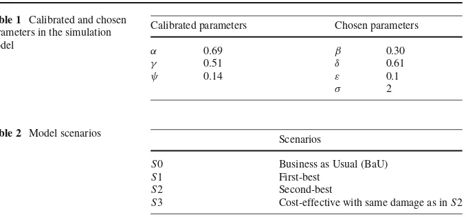
about growth in population, economy and energy use seem to be in between the A1 and the A2 scenarios put forward by the IPCC’s Special Report on Emission Scenarios (IPCC 2000). Based on the other calibration requirements and assumptions above, we can calibrate the remaining model parametersα,γ andψas listed below in Table1. The value ofβis picked.
5.2 Scenarios
We run four alternative scenarios, see Table2. All scenarios have the same stock levels in 2000, and climate change policy is introduced in 2010 in all scenarios exceptS0 (the BaU scenario).S1 andS2 denote the first- and second-best policy scenarios, whereasS3 denotes the cost-effective scenario outlined in Sect. 4. However, instead of assuming a concentration
15Ten years may seem a bit short for the lifetime of patents, as patent length in the US is 17 years and in Europe 20 years. Note, however, that the main results regarding the ratio of efficient tax over Pigouvian tax (cf. Fig.6) are quite similar when we e.g. double the length of the simulation periods.
16This is of course a simplification of the carbon cycle, i.e., the interaction between CO
Table 1 Calibrated and chosen parameters in the simulation model
Calibrated parameters Chosen parameters
α 0.69 β 0.30
γ 0.51 δ 0.61
ψ 0.14 ε 0.1
σ 2
Table 2 Model scenarios Scenarios
S0 Business as Usual (BaU)
S1 First-best
S2 Second-best
S3 Cost-effective with same damage as inS2
ceiling, we apply the following constraint:
∞
0
δtD(St)≤ ∞
0
δtDSt∗, (44)
whereSt∗is the concentration level in theS2 solution. The purpose of introducing this sce-nario is to examine the timing of abatement within a first- and second-best model, where the discounted climate change damage costs are equal. That is,S3 is delivering the least cost emission trajectory with the same discounted damage costs asS2.
5.3 Numerical Results
Figure1shows the development of fossil (Et) and CO2-free (At) energy over the next two
centuries, measured in Gigaton carbon per year (on a logarithmic scale) in the business as usual and the second-best policy. We only show policy scenarioS2, as the policy scenarios
S1, S2, and S3 almost coincide when using the logarithmic scale of Fig.1. In the policy scenarios, we see from Fig.1that fossil energy reaches a top in the middle of this century,
0.0 0.1 1.0 10.0 100.0
2000 2050 2100 2150 2200
Gi
g
aton carbon per year Fossil energy (S0)
CO2-free energy (S0)
Fossil energy (S2)
CO2-free energy (S2)
-15% -10% -5% 0% 5% 10% 15%
2000 2050 2100 2150 2200
S2 vs. S1
S2 vs S3
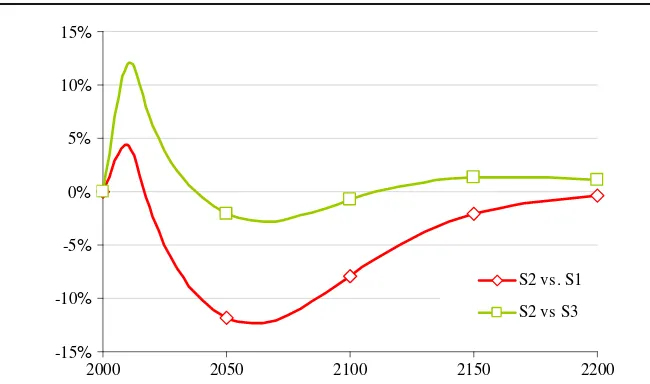
Fig. 2 CO2free energy in second-best versus first-best
and falls below CO2-free energy just before 2100. Comparing the second-best scenarioS2 withS1 andS3 (see Fig.2), we can see the implications of policy having abatement research subsidies available, or not. In general, the absence of a policy instrument raises the social costs of abatement, and thus lowers the aggregate abatement level (S2 vs.S1). But, when there are no abatement research subsidies, efficient carbon taxes will be higher. Therefore, in the first periods when the level of technology is still similar in both scenarios, abatement levels are higher in the second-best policy scenario. The effect is more pronounced when we compareS2 withS3. Making this comparison, the net present value of damages are the same, and the only difference between the scenarios is due to the timing of abatement. We thus see that the second-best policy scenario starts with high carbon taxes and consequently, with high abatement levels. The other way around, with all policy instruments available (S3 vs.
S2, the negative of the upper curve), R&D is shifted upfront, whereas abatement is delayed. The timing issue is also visible in Fig.3, which shows the annual growth rate in CO2-free energy expenditures (i.e., growth inZt+Xt). We notice that in all scenarios the growth rate
falls, that is, the abatement sector is maturing as defined above Proposition 1. The transition from an infant industry into a matured industry is most pronounced in the policy scenar-ios. Obviously, climate change policy increases abatement growth substantially over the first century, but eventually, the CO2-free energy sector matures around the middle of the next century, as it takes over the energy market almost completely. From that time onwards, CO2-free energy expenditures grow at the same rate as total energy use, i.e., by 1% per year. We further notice that growth rates in the scenarios S1 and S3 virtually coincide (in the figure, theS1 curve is hidden behind theS3 curve). When comparing these scenarios with the second-best scenario (S2), we find that expenditures grow slightly faster in the former scenarios throughout the simulation period (thelevelof expenditures starts at a higher level inS2 though).
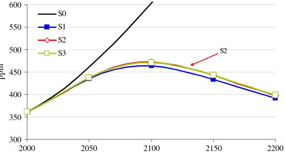
Although we apply only a simple one-box resource model, still it can produce qualitative insights in the concentration level of CO2in the atmosphere (St). The concentration peaks
0,00 0,01 0,02 0,03 0,04 0,05 0,06
2000 2050 2100 2150 2200
Ann
u
al rate of
g
rowh
S0
S1
S2
S3
S1
Fig. 3 Growth in CO2-free energy expenditures in the different scenarios. The arrow points to scenarioS1 that is behind scenarioS3
300 350 400 450 500 550 600
2000 2050 2100 2150 2200
p
p
m
S0
S1
S2
S3 S2
Fig. 4 Concentration level of CO2in the different scenarios. The arrow points to scenarioS2 that is behind scenarioS3.
at a slightly lower level than with a second-best policyS2. The two scenarios with equal net present value of damages,S2 andS3, are very similar.
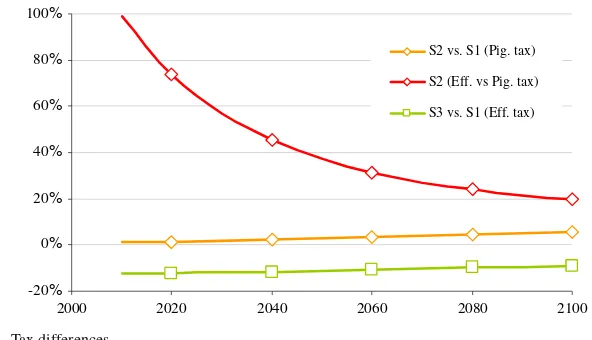
In Figs.5and6we show how the Pigouvian tax (θt) and the efficient tax (τt) develop
in the three policy scenarios. In the first-best scenario (S1), these two taxes are equal (cf. Proposition 1). In the second-best scenario (S2) they are generally not (cf. Eq.38), and in our numerical simulations the efficient tax is well above the Pigouvian tax, almost 100% in 2010, while the relative gap falls monotonically to about 20% in 2100 (Fig.6, “S2 (Eff. versus Pig. tax)”). The lack of policy instruments to directly target R&D has thus very significant effects on the (second-best) tax level. This confirms Proposition 2, which states that the relative difference between the efficient and the Pigouvian tax will fall over time in the case with a maturing abatement sector (see Fig.3).
0 200 400 600 800 1000 1200 1400
2000 2020 2040 2060 2080 2100
E
u
ro/ton carbon
Efficient=Pigouvian tax (S1)
Pigouvian tax (S2)
Efficient tax (S2)
Efficient tax (S3)
Fig. 5 Efficient tax and Pigouvian tax in the different scenarios
-20% 0% 20% 40% 60% 80% 100%
2000 2020 2040 2060 2080 2100
S2 vs. S1 (Pig. tax)
S2 (Eff. vs Pig. tax)
S3 vs. S1 (Eff. tax)
Fig. 6 Tax differences
abatement is required compared to the first-best (S1) (cost-benefit) scenario. Note that in the cost-effective scenario (S3), abatement levels are less than optimal (given the climate change damage function), as the objective is to minimise abatement costs for a fixed present value of future climate change damages (based onS2).
6 Conclusion
of users of R&D models versus users of LbD models. This divergence in perspective arising from the two types of models may be overdone. First, the empirical literature suggests that both R&D and learning by doing play their own role in bringing down the costs of abate-ment (Söderholm and Klaassen 2007;Söderholm and Sundqvist 2006). Second, we find in an analytical framework that also in a pure R&D model, one can find reasons for upfront or delayed abatement efforts, but the difference in results is now based on the availability of policy instruments.
If the public authority can directly steer the development of energy-related technology, either through public energy-related R&D or through targeted private R&D, then it is efficient to spend much of the initial effort on this technological development. In both cases it is to be noted that in the phase of the emerging climate change problem, substantial public funds are to be directed to developing emission reducing technologies, either through public R&D or through high subsidies on private R&D (Proposition 1).
However, if the public authority cannot directly determine the development of an emission reducing technology, then efficiency considerations suggest that the clean technology should be extra stimulated through an increased demand for its produced goods. The technology pull policy should be relatively strong during the emerging phase of the climate change problem, when the abatement technologies still have to mature. The major feature responsible for this result is an assumed finite lifetime of patents. The numerical simulations suggest that this may translate into a significantly higher tax on CO2than in a first-best scenario.
As a final comment, we notice that the theoretical analysis we carried out has been fairly general, so that our findings may imply more generally that infant industries should be stim-ulated to a larger degree than mature industries. This topic may be worked out in future research.
Acknowledgements Comments from Rolf Golombek, Michael Hoel, and many other participants in the project “Environmental economics: policy instruments, technology development, and international cooper-ation”, as well as three anonymous referees are gratefully acknowledged. The research for this paper was for a large part conducted at the Centre for Advanced Study (CAS) at the Norwegian Academy of Science and Letters in Oslo in 2005/2006. The financial, administrative and professional support of the Centre to this project is much appreciated. There has also been some additional funding. Gerlagh would like to thank the Dutch NWO Vernieuwingsimpuls program for support, and Kverndokk and Rosendahl would like to thank the programme RENERGI at the Research Council of Norway for financial support.
References
Barro R, Sala-i-Martin X (1995) Economic growth. The MIT Press, Cambridge, Massachusetts
Bovenberg AL, de Mooij RA (1994) Environmental levies and distortionary taxation. Am Econ Rev 84:1085– 1089
BP Statistical Review of World Energy. June 2006.http://www.bp.com/productlanding.do?categorupId=6929 &contentId=7044622
Bramoulle Y, Olson LJ (2005) Allocation of pollution abatement under learning by doing. J Public Econ 89:1935–1960
Chou C, Shy O (1993) The crowding-out effects of long duration of patents. Rand J Econ 24(2):304–312 Dixit A, Stiglitz JE (1977) Monopolistic competition and optimum product diversity. Am Econ Rev 67:297–
308
Encaoua D, Ulph D (2004) Catching-up or leapfrogging? The effects of competition on innovation and growth. Updated version of report 2000.97. Economie Mathematique et Applications, Paris
Gerlagh R, Lise W (2005) Carbon taxes: a drop in the ocean, or a drop that erodes the stone? The effect of carbon taxes on technological change. Ecol Econ 54:241–260
Gerlagh R, Kverndokk S, Rosendahl KE (2008) Linking environmental and innovation policy, Nota di Lavoro 53.2008, FEEM—Fondazione Eni Enrico Mattei
Golombek R, Hoel M (2005) Climate policy under technology spillover. Environ Res Econ 31:201–227 Goulder LH, Mathai K (2000) Optimal CO2 abatement in the presence of induced technological change.
J Environ Econ Manag 39:1–38
Greaker M, Pade L-L, Optimal CO2abatement and technological change—should emission taxes start high to spur R&D? Discussion paper 548, Statistics Norway, Norway
Grübler A, Messner S (1998) Technological change and the timing of mitigation measures. Energy Econ 20:495–512
Ha-Duong M, Grubb MJ, Hourcade JC (1997) Influence of socioeconomic inertia and uncertainty on optimal CO2-emission abatement. Nature 390:270–273
Hartman R, Kwon OS (2005) Sustainable growth and the environmental Kuznets curve. J Econ Dyn Control 29:1701–1736
Hart R (2008) The timing of taxes on CO2emissions when technological change is endogenous. J Env Econ Manag 55:194–212
Hoel M (1996) Should a carbon tax be differentiated across sectors. J Public Econ 59:17–32 IEA (2002) Renewables information 2002. OECD/IEA, Paris
IEA (2005) World energy outlook 2005. OECD/IEA, Paris
IPCC (1995) Climate change 1994. Radiative forcing of climate change and an evaluation of the IPCC IS92 emission scenarios. Cambridge University Press, Cambridge, United Kingdom and New York, USA IPCC (2000) Special report on emissions scenarios (SRES). Cambridge University Press. Cambridge, United
Kingdom and New York, USA
IPCC (2007) Climate change 2007: The physical science basis. Contribution of working group I to the fourth assessment report of the intergovernmental panel on climate change. Cambridge University Press: Cambridge, United Kingdom and New York, USA
Isoard S, Soria A (2001) Technical change dynamics: evidence from the emerging renewable energy technol-ogies. Energy Econ 23:619–636
Iwaisako T, Futagami K (2003) Patent policy in an endogenous growth model. J Econ 78:239–258 Judd KL (1985) On the performance of patents. Econometrica 53:567–585
Knapp KE (1999) Exploring energy technology substitution for reducing atmoshperic carbon emissions. Energy J 20(2):121–143
Kverndokk S, Rosendahl KE, Rutherford TF (2004) Climate policies and induced technological change: which to choose, the carrot or the stick?. Environ Res Econ 27(1):21–41
Kverndokk S, Rosendahl KE (2007) Climate policies and learning by doing: impacts and timing of technology subsidies. Res Energy Econ 29:58–82
Lieberman MB (1984) The learning curve and pricing in the chemical processing industries. Rand J Econ 15:213–228
Liski M (2002) Taxing average emissions to overcome the shutdown problem. J Public Econ 85:363–384 Manne A, Richels R (2004) The impact of learning-by-doing on the timing and costs of CO2abatement.
Energy Econ (Special Issue) 26:603–619
Nordhaus WD (1969) Theory of innovation, an economic theory of technological change. Am Econ Rev 59:18–28
Nordhaus WD (2002) Modeling induced innovation in climate-change policy. In: Grübler A, Nakicenovic N, Nordhaus WD (eds), Modeling induced innovation in climate-change policy, Chap. 9. Resources for the Future Press, Washington
Popp D (2004) ENTICE: endogenous technological change in the DICE model of global warming. J Environ Econ Manag 48:742–768
Rivers N, Jaccard M (2006) Choice of environmental policy in the presence of learning by doing. Energy Econ 28:223–242
Romer PM (1987) Growth based on increasing returns due to specialization. Am Econ Rev 77(2):56–62 Romer PM (1990) Endogenous technological change. J Polit Econ 98(5):71–102
Rosendahl KE (2004) Cost-effective environmental policy: implications of induced technological change. J Environ Econ Manag 48:1099–1121
Söderholm P, Klaassen G (2007) Wind power in Europe: a simultaneous innovation-diffusion model. Energy Res Econ 36:163–190
Söderholm P, Sundqvist T (2006) Empirical challenges in the use of learning curves for assessing the economic prospects of renewable energy technologies. Renew Energy 32:2559–2578
van der Zwaan BCC, Gerlagh R, Klaassen GAJ, Schrattenholzer L (2002) Endogenous technological change in climate change modelling. Energy Econ 24:1–19