Electric
Circuits
Seventh Edition
Mahmood Nahvi, PhD
Professor Emeritus of Electrical Engineering
California Polytechnic State University
Joseph A. Edminister
Professor Emeritus of Electrical Engineering
The University of Akron
Schaum’s Outline Series
ISBN: 978-1-26-001197-5
MHID: 1-26-001197-6
The material in this eBook also appears in the print version of this title: ISBN: 978-1-26-001196-8,
MHID: 1-26-001196-8.
eBook conversion by codeMantra
Version 1.0
All trademarks are trademarks of their respective owners. Rather than put a trademark symbol after every occurrence of a
trade-marked name, we use names in an editorial fashion only, and to the benefit of the trademark owner, with no intention of infringe
-ment of the trademark. Where such designations appear in this book, they have been printed with initial caps.
McGraw-Hill Education eBooks are available at special quantity discounts to use as premiums and sales promotions or for use in
corporate training programs. To contact a representative, please visit the Contact Us page at www.mhprofessional.com.
Trademarks: McGraw-Hill Education, the McGraw-Hill Education logo, Schaum’s, and related trade dress are trademarks or
registered trademarks of McGraw-Hill Education and/or its affiliates in the United States and other countries, and may not be
used without written permission. All other trademarks are the property of their respective owners. McGraw-Hill Education is not
associated with any product or vendor mentioned
in this book.
TERMS OF USE
This is a copyrighted work and McGraw-Hill Education and its licensors reserve all rights in and to the work. Use of this work
is subject to these terms. Except as permitted under the Copyright Act of 1976 and the right to store and retrieve one copy of the
work, you may not decompile, disassemble, reverse engineer, reproduce, modify, create derivative works based upon, transmit,
distribute, disseminate, sell, publish or sublicense the work or any part of it without McGraw-Hill Education’s prior consent. You
may use the work for your own noncommercial and personal use; any other use of the work is strictly prohibited. Your right to use
the work may be terminated if you fail to comply with these terms.
iii
The seventh edition of
Schaum’s Outline of Electric Circuits
represents a revision and timely update of
materials that expand its scope to the level of similar courses currently taught at the undergraduate level.
The new edition expands the information on the frequency response, polar and Bode diagrams, and first-
and second-order filters and their implementation by active circuits. Sections on lead and lag networks
and filter analysis and design, including approximation method by Butterworth filters, have been added,
as have several end-of-chapter problems.
The original goal of the book and the basic approach of the previous editions have been retained. This
book is designed for use as a textbook for a first course in circuit analysis or as a supplement to standard
texts and can be used by electrical engineering students as well as other engineering and technology
stu-dents. Emphasis is placed on the basic laws, theorems, and problem-solving techniques that are common
to most courses.
The subject matter is divided into 17 chapters covering duly recognized areas of theory and study. The
chapters begin with statements of pertinent definitions, principles, and theorems together with
illustra-tive examples. This is followed by sets of supplementary problems. The problems cover multiple levels
of difficulty. Some problems focus on fine points and help the student to better apply the basic principles
correctly and confidently. The supplementary problems are generally more numerous and give the reader
an opportunity to practice problem-solving skills. Answers are provided with each supplementary problem.
The book begins with fundamental definitions, circuit elements including dependent sources, circuit
laws and theorems, and analysis techniques such as node voltage and mesh current methods. These
theo-rems and methods are initially applied to DC-resistive circuits and then extended to RLC circuits by the use
of impedance and complex frequency. The op amp examples and problems in Chapter 5 have been selected
carefully to illustrate simple but practical cases that are of interest and importance to future courses. The
subject of waveforms and signals is treated in a separate chapter to increase the student’s awareness of
commonly used signal models.
Circuit behavior such as the steady state and transient responses to steps, pulses, impulses, and
expo-nential inputs is discussed for first-order circuits in Chapter 7 and then extended to circuits of higher order
in Chapter 8, where the concept of complex frequency is introduced. Phasor analysis, sinusoidal steady
state, power, power factor, and polyphase circuits are thoroughly covered. Network functions, frequency
response, filters, series and parallel resonance, two-port networks, mutual inductance, and transformers are
covered in detail. Application of Spice and PSpice in circuit analysis is introduced in Chapter 15. Circuit
equations are solved using classical differential equations and the Laplace transform, which permits a
con-venient comparison. Fourier series and Fourier transforms and their use in circuit analysis are covered in
Chapter 17. Finally, two appendixes provide a useful summary of complex number systems and matrices
and determinants.
This book is dedicated to our students and students of our students, from whom we have learned to teach
well. To a large degree, it is they who have made possible our satisfying and rewarding teaching careers.
We also wish to thank our wives, Zahra Nahvi and Nina Edminister, for their continuing support. The
con-tribution of Reza Nahvi in preparing the current edition as well as previous editions is also acknowledged.
M
AHMOODN
AHVIMAHMOOD NAHVI is professor emeritus of Electrical Engineering at California Polytechnic State University in San Luis Obispo, California. He earned his B.Sc., M.Sc., and Ph.D., all in electrical engineering, and has 50 years of teaching and research in this field. Dr. Nahvi’s areas of special interest and expertise include network theory, control theory, communications engineering, signal processing, neural networks, adaptive control and learning in synthetic and living systems, communication and control in the central nervous system, and engineering education. In the area of engineering education, he has developed computer modules for electric circuits, signals, and systems which improve teaching and learning of the fundamentals of electrical engineering. In addition, he is coauthor of Electromagnetics in Schaum’s Outline Series, and the author of Signals and Systems published by McGraw-Hill.
v
CHAPTER 1 Introduction
1
1.1
Electrical Quantities and SI Units
1.2
Force, Work, and Power
1.3
Electric Charge and Current
1.4
Electric Potential
1.5
Energy and
Electrical Power
1.6
Constant and Variable Functions
CHAPTER 2 Circuit Concepts
7
2.1
Passive and Active Elements
2.2
Sign Conventions
2.3
Voltage-Current
Relations
2.4
Resistance
2.5
Inductance
2.6
Capacitance
2.7
Circuit
Diagrams
2.8
Nonlinear Resistors
CHAPTER 3 Circuit Laws
24
3.1
Introduction
3.2
Kirchhoff’s Voltage Law
3.3
Kirchhoff’s Current
Law
3.4
Circuit Elements in Series
3.5
Circuit Elements in Parallel
3.6
Voltage Division
3.7
Current Division
CHAPTER 4 Analysis Methods
37
4.1
The Branch Current Method
4.2
The Mesh Current Method
4.3
Matrices and Determinants
4.4
The Node Voltage Method
4.5
Network
Reduction
4.6
Input Resistance
4.7
Output Resistance
4.8
Transfer
Resistance
4.9
Reciprocity Property
4.10
Superposition
4.11
Thévenin’s
and Norton’s Theorems
4.12
Maximum Power Transfer Theorem
4.13
Two-Terminal Resistive Circuits and Devices
4.14
Interconnecting
Two-Terminal Resistive Circuits
4.15
Small-Signal Model of Nonlinear
Resistive Devices
CHAPTER 5 Amplifiers and Operational Amplifier Circuits
72
5 . 1
Amplifier Model
5 . 2
Feedback in Amplifier Circuits
5.3
Operational Amplifiers
5.4
Analysis of Circuits Containing Ideal Op
Amps
5.5
Inverting Circuit
5.6
Summing Circuit
5.7
Noninverting
Circuit
5.8
Voltage Follower
5.9
Differential and Difference Amplifiers
5.10
Circuits Containing Several Op Amps
5.11
Integrator and
Differentiator Circuits
5.12
Analog Computers
5.13
Low-Pass Filter
5.14
Decibel (dB)
5.15
Real Op Amps
5.16
A Simple Op Amp
Model
5.17
Comparator
5.18
Flash Analog-to-Digital Converter
5.19
Summary of Feedback in Op Amp Circuits
CHAPTER 6 Waveforms and Signals
117
6.1
Introduction
6.2
Periodic Functions
6.3
Sinusoidal Functions
6.4
Time Shift and Phase Shift
6.5
Combinations of Periodic Functions
6.6
The Average and Effective (RMS) Values
6.7
Nonperiodic Functions
6.8
The Unit Step Function
6.9
The Unit Impulse Function
6.10
The
Exponential Function
6.11
Damped Sinusoids
6.12
Random Signals
CHAPTER 7 First-Order Circuits
143
7.1
Introduction
7.2
Capacitor Discharge in a Resistor
7.3
Establishing
a DC Voltage Across a Capacitor
7.4
The Source-Free
RL
Circuit
7.5
Establishing a DC Current in an Inductor
7.6
The Exponential
Function Revisited
7.7
Complex First-Order
RL
and
RC
Circuits
7.8
DC
Steady State in Inductors and Capacitors
7.9
Transitions at Switching Time
7.10
Response of First-Order Circuits to a Pulse
7.11
Impulse Response
of
RC
and
RL
Circuits
7.12
Summary of Step and Impulse Responses
in
RC
and
RL
Circuits
7.13
Response of
RC
and
RL
Circuits to Sudden
Exponential Excitations
7.14
Response of
RC
and
RL
Circuits to Sudden
Sinusoidal Excitations
7.15
Summary of Forced Response in First-Order
Circuits
7.16
First-Order Active Circuits
CHAPTER 8 Higher-Order Circuits and Complex Frequency
179
8.1
Introduction
8.2
Series
RLC
Circuit
8.3
Parallel
RLC
Circuit
8.4
Two-Mesh Circuit
8.5
Complex Frequency
8.6
Generalized
Impedance (
R
,
L
,
C
) in s-Domain
8.7
Network Function and Pole-Zero
Plots
8.8
The Forced Response
8.9
The Natural Response
8.
1
0
Magnitude
and Frequency Scaling
8.
1
1
Higher-Order Active Circuits
CHAPTER 9 Sinusoidal Steady-State Circuit Analysis
209
9.1
Introduction
9.2
Element Responses
9.3
Phasors
9.4
Impedance
and Admittance
9.5
Voltage and Current Division in the Frequency
Domain
9.6
The Mesh Current Method
9.7
The Node Voltage
Method
9.8
Thévenin’s and Norton’s Theorems
9.9
Superposition of AC
Sources
CHAPTER 10 AC Power
237
10.1
Power in the Time Domain
10.2
Power in Sinusoidal Steady
State
10.3
Average or Real Power
10.4
Reactive Power
10.5
Summary
of AC Power in
R
,
L
, and
C
10.6
Exchange of Energy between an Inductor
and a Capacitor
10.7
Complex Power, Apparent Power, and Power Triangle
10.8
Parallel-Connected Networks
10.9
Power Factor Improvement
10.10
Maximum Power Transfer
10.11
Superposition of Average Powers
CHAPTER 11 Polyphase Circuits
266
11.1
Introduction
11.2
Two-Phase Systems
11.3
Three-Phase Systems
11.4
Wye and Delta Systems
11.5
Phasor Voltages
11.6
Balanced
Delta-Connected Load
11.7
Balanced Four-Wire, Wye-Connected Load
for Balanced Three-Phase Loads
11.10
Unbalanced Delta-Connected
Load
11.11
Unbalanced Wye-Connected Load
11.12
Three-Phase
Power
11.13
Power Measurement and the Two-Wattmeter Method
CHAPTER 12 Frequency Response, Filters, and Resonance
291
12.1
Frequency Response
12.2
High-Pass and Low-Pass Networks
12.3
Half-Power Frequencies
12.4
Generalized Two-Port, Two-Element
Networks
12.5
The Frequency Response and Network Functions
12.6
Frequency Response from Pole-Zero Location
12.7
Ideal and
Practical Filters
12.8
Passive and Active Filters
12.9
Bandpass Filters
and Resonance
12.10
Natural Frequency and Damping Ratio
12.11
RLC
Series Circuit; Series Resonance
12.12
Quality Factor
12.13
RLC
Parallel
Circuit; Parallel Resonance
12.14
Practical
LC
Parallel Circuit
12.15
Series-Parallel Conversions
12.16
Polar Plots and Locus Diagrams
12.17
Bode
Diagrams
12.18
Special Features of Bode Plots
12.19
First-Order
Filters
12.20
Second-Order Filters
12.21
Filter Specifications;
Bandwidth, Delay, and Rise Time
12.22
Filter Approximations: Butterworth
Filters
12.23
Filter Design
12.24
Frequency Scaling and Filter
Transformation
CHAPTER 13 Two-Port Networks
344
13.1
Terminals and Ports
13.2
Z
-Parameters
13.3
T-Equivalent of
Reciprocal Networks
13.4
Y-Parameters
13.5
Pi-Equivalent of Reciprocal
Networks
13.6
Application of Terminal Characteristics
13.7
Conversion
between Z- and Y-Parameters
13.8
h-Parameters
13.9
g-Parameters
13.10
Transmission Parameters
13.11
Interconnecting Two-Port Networks
13.12
Choice of Parameter Type
13.13
Summary of Terminal Parameters
and Conversion
CHAPTER 14 Mutual Inductance and Transformers
368
14.1
Mutual Inductance
14.2
Coupling Coefficient
14.3
Analysis of
Coupled Coils
14.4
Dot Rule
14.5
Energy in a Pair of Coupled Coils
14.6
Conductively Coupled Equivalent Circuits
14.7
Linear Transformer
14.8
Ideal Transformer
14.9
Autotransformer
14.10
Reflected
Impedance
CHAPTER 15 Circuit Analysis Using Spice and PSpice
396
15.1
Spice and PSpice
15.2
Circuit Description
15.3
Dissecting a Spice
Source File
15.4
Data Statements and DC Analysis
15.5
Control and Output
Statements in DC Analysis
15.6
Thévenin Equivalent
15.7
Subcircuit
15.8
Op Amp Circuits
15.9
AC Steady State and Frequency Response
15.10
Mutual Inductance and Transformers
15.11
Modeling Devices
with Varying Parameters
15.12
Time Response and Transient Analysis
15.13
Specifying Other Types of Sources
15.14
Summary
CHAPTER 16 The Laplace Transform Method
434
CHAPTER 17 Fourier Method of Waveform Analysis
457
17.1
Introduction
17.2
Trigonometric Fourier Series
17.3
Exponential
Fourier Series
17.4
Waveform Symmetry
17.5
Line Spectrum
17.6
Waveform Synthesis
17.7
Effective Values and Power
17.8
Applications
in Circuit Analysis
17.9
Fourier Transform of Nonperiodic Waveforms
17.10
Properties of the Fourier Transform
17.11
Continuous Spectrum
APPENDIX A Complex Number System
491
APPENDIX B Matrices and Determinants
494
1
Introduction
1.1 Electrical Quantities and SI Units
The International System of Units (SI) will be used throughout this book. Four basic quantities and their SI
units are listed in Table 1-1. The other three basic quantities and corresponding SI units, not shown in the
table, are temperature in degrees kelvin (K), amount of substance in moles (mol), and luminous intensity in
candelas (cd).
All other units may be derived from the seven basic units. The electrical quantities and their symbols
commonly used in electrical circuit analysis are listed in Table 1-2.
Two supplementary quantities are plane angle (also called phase angle in electric circuit analysis) and
solid angle. Their corresponding SI units are the radian (rad) and steradian (sr).
Degrees are almost universally used for the phase angles in sinusoidal functions, as in, sin(
w
t
+
30
°
).
(Since
wt
is in radians, this is a case of mixed units.)
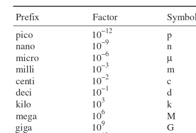
The decimal multiples or submultiples of SI units should be used whenever possible. The symbols given
in Table 1-3 are prefixed to the unit symbols of Tables 1-1 and 1-2. For example, mV is used for millivolt,
10
−3V, and MW for megawatt, 10
6W.
Table 1-1
Quantity Symbol SI Unit Abbreviation length
Quantity Symbol SI Unit Abbreviation
1.2 Force, Work, and Power
The derived units follow the mathematical expressions which relate the quantities. From ‘‘force equals mass
times acceleration,’’ the
newton
(N) is defined as the unbalanced force that imparts an acceleration of 1 meter
per second squared to a 1-kilogram mass. Thus, 1N
=
1 kg · m/s
2.
Work results when a force acts over a distance. A
joule
of work is equivalent to a
newton-meter
: 1 J
=
1 N · m. Work and energy have the same units.
Power is the rate at which work is done or the rate at which energy is changed from one form to another.
The unit of power, the
watt
(W), is one joule per second (J/s).
EXAMPLE 1.1 In simple rectilinear motion, a 10-kg mass is given a constant acceleration of 2.0 m/s2. (a) Find the acting force F. (b) If the body was at rest at t = 0, x = 0, find the position, kinetic energy, and power for t = 4 s.
1.3 Electric Charge and Current
The unit of current, the
ampere
(A), is defined as the constant current in two parallel conductors of infinite
length and negligible cross section, 1 meter apart in vacuum, which produces a force between the conductors
of 2.0
×
10
−7newtons per meter length. A more useful concept, however, is that current results from charges
in motion, and 1 ampere is equivalent to 1 coulomb of charge moving across a fixed surface in 1 second. Thus,
in time-variable functions,
i
(A)
=
dq
/
dt
(C/s). The derived unit of charge, the
coulomb
(C), is equivalent to an
ampere-second.
The moving charges may be positive or negative. Positive ions, moving to the left in a liquid or plasma
suggested in Fig. 1-1(
a
), produce a current
i
, also directed to the left. If these ions cross the plane surface
S
at the rate of
one coulomb per second
, then the resulting current is 1 ampere. Negative ions moving to the
right as shown in Fig. 1-1(
b
) also produce a current directed to the left.
so that for a current of one ampere approximately 6.24
×
10
18electrons per second would have to pass a fixed
cross section of the conductor.
EXAMPLE 1.2 A conductor has a constant current of 5 amperes. How many electrons pass a fixed point on the con-ductor in 1 minute?
5 5
1 602
A C/s 60 s/min 300 C/min 300 C/min
= =
×
( )( )
. 110 19 1 87 10 21
− = ×
C/electron . electrons/min
1.4 Electric Potential
An electric charge experiences a force in an electric field which, if unopposed, will accelerate the charge. Of
interest here is the work done to move the charge against the field as suggested in Fig. 1-2(
a
). Thus, if
1
joule
of work is required to move the
1
coulomb
charge
Q
, from position 0 to position 1, then position 1 is at a potential
of
1
volt
with respect to position 0; 1 V
=
1 J/C. This electric potential is capable of doing work just as the
mass in Fig. 1-2(
b
), which was raised against the gravitational force
g
to a height
h
above the ground plane.
The potential energy
mgh
represents an ability to do work when the mass
m
is released. As the mass falls, it
accelerates and this potential energy is converted to kinetic energy.
Fig. 1-1
Fig. 1-2
EXAMPLE 1.3 In an electric circuit, an energy of 9.25 µJ is required to transport 0.5 µC from point a to point b. What electric potential difference exists between the two points?
1 1 9 25 10
10 6
volt joule per coulomb J
0.5
= = ×
×
−
1.5 Energy and Electrical Power
Electric energy in joules will be encountered in later chapters dealing with capacitance and induc tance whose
respective electric and magnetic fields are capable of storing energy. The rate, in
joules per second
, at which
energy is transferred is electric power in
watts
. Furthermore, the product of voltage and current yields
the electric power,
p
=
ni
; 1 W
=
1 V · 1 A. Also, V · A
=
(J/C) · (C/s)
=
J/s
=
W. In a more fundamental
sense power is the time derivative
p
=
dw
/
dt
, so that instantaneous power
p
is generally a function of time.
In the following chapters time average power
P
avgand a root-mean-square (RMS) value for the case where
voltage and current are sinusoidal will be developed.
EXAMPLE 1.4 A resistor has a potential difference of 50.0 V across its terminals and 120.0 C of charge per minute passes a fixed point. Under these conditions at what rate is electric energy converted to heat?
(120.0 C/min)/(60 s/min)=2.0 A P=(2.0 A)(50.00 V)=100.0 W Since 1 W = 1 J/s, the rate of energy conversion is 100 joules per second.
1.6 Constant and Variable Functions
To distinguish between constant and time-varying quantities, capital letters are employed for the constant
quantity and lowercase for the variable quantity. For example, a constant current of 10 amperes is written
I
=
10.0 A, while a 10-ampere time-variable current is written
i
=
10.0
f
(
t
) A. Examples of common
func-tions in circuit analysis are the sinusoidal function
i
=
10.0 sin
wt
(A) and the exponential function
n
=
15.0
e
−at(V).
SOLVED PROBLEMS
1.1
The force applied to an object moving in the
x
direction varies according to
F
=
12/
x
2(N). (
a
) Find the
work done in the interval 1 m
≤
x
≤
3 m. (
b
) What constant force acting over the same interval would
result in the same work?
(a) dW F dx W
1.2
Electrical energy is converted to heat at the rate of 7.56 kJ/min in a resistor which has 270 C/min
passing through. What is the voltage difference across the resistor terminals?
From
P = VI
,
energy
W
Ttransferred in one period of the sine function.
Energy is the time-integral of instantaneous power:
WT =
∫
υi dt=∫
ωt dt= ω πThe average power is then
Pavg WT
/ mW
= =
1.4
The unit of energy commonly used by electric utility companies is the kilowatt-hour (kWh). (
a
) How
many joules are in 1 kWh? (
b
) A color television set rated at 75 W is operated from 7:00 p.m. to 11:30 p.m.
What total energy does this represent in kilowatt-hours and in mega-joules?
(a) 1 kWh = (1000 J/s)(3600 s) = 3.6 MJ
(b) (75.0 W)(4.5 h) = 337.5 Wh = 0.3375 kWh
(0.3375 kWh)(3.6 MJ/kWh) = 1.215 MJ
1.5
An AWG #12 copper wire, a size in common use in residential wiring, contains approximately 2.77
×
10
23free electrons per meter length, assuming one free conduction electron per atom. What percentage of these
electrons will pass a fixed cross section if the conductor carries a constant current of 25.0 A?
25.0 C/s
1.602 10 C/electron 1.56 10 elect 20
× −19 = × rron/s
(1.56×10²⁰ electron/s)(60 s/min)=9 36. ×11021electrons/min 9.36 10
2.77 10 (100) 3 21
23
×
× = ..38%
1.6
How many electrons pass a fixed point in a 100-watt light bulb in 1 hour if the applied constant voltage
is 120 V?
100 120
3600
W V A 5/6 A
5/6 C/s
=( )× ( ) =
( )(
I I
ss/h
C/electron electr )
. .
1 602 10 19 1 87 10 22
× − = × oons per hour
1.7
A typical 12 V auto battery is rated according to
ampere-hours
. A 70-A · h battery, for example, at a
discharge rate of 3.5 A has a life of 20 h. (
a
) Assuming the voltage remains constant, obtain the energy
and power delivered in a complete discharge of the preceding battery. (
b
) Repeat for a discharge rate
of 7.0 A.
(a) (3.5 A)(12 V) = 42.0 W (or J/s)
(42.0 J/s)(3600 s/h)(20 h) = 3.02 MJ (b) (7.0 A)(12 V) = 84.0 W
(84.0 J/s)(3600 s/h)(10 h) = 3.02 MJ
The ampere-hour rating is a measure of the energy the battery stores; consequently, the energy
trans-ferred for total discharge is the same whether it is transtrans-ferred in 10 hours or 20 hours. Since power is
the rate of energy transfer, the power for a 10-hour discharge is twice that in a 20-hour discharge.
SUPPLEMENTARY PROBLEMS
1.8 Obtain the work and power associated with a force of 7.5 × 10⁻⁴ N acting over a distance of 2 meters in an elapsed time of 14 seconds. Ans. 1.5 mJ, 0.107 mW
1.9 Obtain the work and power required to move a 5.0-kg mass up a frictionless plane inclined at an angle of 30° with the horizontal for a distance of 2.0 m along the plane in a time of 3.5 s. Ans. 49.0 J, 14.0 W
1.10 Work equal to 136.0 joules is expended in moving 8.5 × 10¹⁸ electrons between two points in an electric circuit. What potential difference does this establish between the two points? Ans. 100 V
1.11 A pulse of electricity measures 305 V, 0.15 A, and lasts 500 µs. What power and energy does this represent?
Ans. 45.75 W, 22.9 mJ
1.13 For t ≥ 0, q = (4.0 × 10⁻⁴)(1 − e−250t) (C). Obtain the current at t = 3 ms. Ans. 47.2 mA 1.14 A certain circuit element has the current and voltage
i
=
10
e
−5000t( )
A
υ
=
50 1
(
−
e
−5000t) ( )
V
Find the total energy transferred during t ≥ 0. Ans. 50 mJ1.15 The capacitance of a circuit element is defined as Q/V, where Q is the magnitude of charge stored in the element and V is the magnitude of the voltage difference across the element. The SI derived unit of capacitance is the
7
Circuit Concepts
2.1 Passive and Active Elements
An electrical device is represented by a
circuit diagram
or
network
constructed from series and parallel
arrangements of two-terminal elements. The analysis of the circuit diagram predicts the performance of the
actual device. A two-terminal element in general form is shown in Fig. 2-1, with a single device represented
by the rectangular symbol and two perfectly conducting leads ending at connecting points
A
and
B. Active
elements are voltage or current sources which are able to supply energy to the network. Resistors, inductors,
and capacitors are
passive
elements which take energy from the sources and either convert it to another form
or store it in an electric or magnetic field.
Fig. 2-1
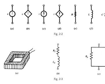
Figure 2-2 illustrates seven basic circuit elements. Elements (
a
)
and (
b
)
are voltage sources and
(
c
)
and (
d
)
are current sources. A voltage source that is not affected by changes in the connected
circuit is an
independent
source, illustrated by the circle in Fig. 2-2(
a
)
.
A
dependent
voltage source
which changes in some described manner with the conditions on the connected circuit is shown by the
diamond-shaped symbol in Fig. 2-2(
b
)
.
Current sources may also be either independent or dependent
and the corresponding symbols are shown in (
c
)
and (
d
)
.
The three passive circuit elements are shown
in Fig. 2-2(
e
), (
f
), and (
g
)
.
The circuit diagrams presented here are termed
lumped-parameter
circuits, since a single element in
one location is used to represent a distributed resistance, inductance, or capacitance. For example, a coil
consisting of a large number of turns of insulated wire has resistance throughout the entire length of the
wire. Nevertheless, a single resistance
lumped
at one place as in Fig. 2-3(
b
) or (
c
)
represents the distributed
resistance. The inductance is likewise lumped at one place, either in series with the resistance as in (
b
)
or in
parallel as in (
c
)
.
2.2 Sign Conventions
A voltage function and a polarity must be specified to completely describe a voltage source. The polarity
marks,
+
and
−
, are placed near the conductors of the symbol that identifies the voltage source. If, for example,
u
=
10.0 sin
w
t
in Fig. 2-4(
a
)
,
terminal
A
is positive with respect to
B
for 0 <
w
t
<
p
,
and
B
is positive with
respect to
A
for
p
<
w
t
<
2
p
for the first cycle of the sine function.
Fig. 2-2
Fig. 2-3
Fig. 2-4
Similarly, a current source requires that a direction be indicated, as well as the function, as shown in
Fig. 2-4(
b
)
.
For passive circuit elements
R
,
L
, and
C
, shown in Fig. 2-4(
c
), the terminal where the current
enters is generally treated as positive with respect to the terminal where the current leaves.
2.3 Voltage-Current Relations
The passive circuit elements resistance
R
, inductance
L
, and capacitance
C
are defined by the manner
in which the voltage and current are related for the individual element. For example, if the voltage
u
and current
i
for a single element are related by a constant, then the element is a resistance,
R
is the
constant of proportionality, and
u
=
Ri
. Similarly, if the voltage is proportional to the time derivative
of the current, then the element is an inductance,
L
is the constant of proportionality, and
u
=
L
di
/
dt
.
Finally, if the current in the element is proportional to the time derivative of the voltage, then the
ele-ment is a capacitance,
C
is the constant of proportionality, and
i
=
C
d
u
/
dt
. Table 2-1 summarizes these
relationships for the three passive circuit elements. Note the current directions and the corresponding
polarity of the voltages.
Fig. 2-5
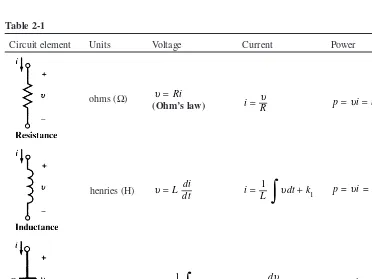
Table 2-1
Circuit element Units Voltage Current Power
ohms (Ω) υ= Ri
(Ohm’s law) i= Rυ p=υi=i R2
henries (H) υ=L di
dt i= L
∫
dt+k 11
υ p i Lidi
dt =υ =
farads (F) υ= 1 2
C
∫
i dt+k i C ddt
= υ p i C d
2.4 Resistance
All electrical devices that consume energy must have a resistor (also called a
resistance
) in their circuit
model. Inductors and capacitors may store energy but over time return that energy to the source or to another
circuit element. Power in the resistor, given by
p
=
u
i
=
i
2R
=
u
2/
R
, is always positive as illustrated in
Example 2.1 below. Energy is then determined as the integral of the instantaneous power
w
p dt
R
i dt
R
dt
t t
t t
t t
=
∫
=
∫
=
∫
1 2
1 2
1 2 2
1
υ
2EXAMPLE 2.1 A 4.0-Ω resistor has a current i =2.5 sin w t (A). Find the voltage, power, and energy over one cycle, given that w =500 rad/s.
υ ω
υ ω
=
= =
Ri t
p i i R t
=
=
10.0 sin (V) 25.0 sin (W)
2 2
w
w p dt t t
t
= = −
(
)
∫
25 02 2 4 0
. sin ω
ω J
The plots of i, p, and w shown in Fig. 2-6 illustrate that p is always positive and that the energy w, although a function of time, is always increasing. This is the energy absorbed by the resistor.
2.5 Inductance
The circuit element that stores energy in a magnetic field is an inductor (also called an
inductance
). With
time-variable current, the energy is generally stored during some parts of the cycle and then returned to the
source during others. When the inductance is removed from the source, the magnetic field will collapse; in
other words, no energy is stored without a connected source. Coils found in electric motors, transformers, and
similar devices can be expected to have inductances in their circuit models. Even a set of parallel conductors
exhibits inductance that must be considered at most frequencies. The power and energy relationships are as
follows.
p
i
L
di
dt
i
d
dt
Li
=
=
=
υ
1
2
2w
Lp dt
Li di
L i
i
t t
i i
=
∫
=
∫
=
−
1 2
1
2
1
2
22 1 2
Energy stored in the magnetic field of an inductance is
w
L=
12Li
2.
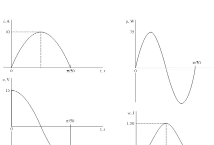
EXAMPLE 2.2 In the interval 0 < t < (p /50)s a 30-mH inductance has a current i =10.0 sin 50t (A). Obtain the voltage, power, and energy for the inductance.
υ=Ldi = =υ =
dt 15.0cos 50t( )V p i 75.0 sin 100 (W)t wwL p dt t t
=
∫
=0 75 1− 100 0. ( cos ) ( )J
As shown in Fig. 2-7, the energy is zero at t =0 and t =(p /50) s. Thus, while energy transfer did occur over the interval, this energy was first stored and later returned to the source.
2.6 Capacitance
The circuit element that stores energy in an electric field is a
capacitor
(also called
capacitance
). When the
voltage is variable over a cycle, energy will be stored during one part of the cycle and returned in the next.
While an inductance cannot retain energy after removal of the source because the magnetic field collapses,
the capacitor retains the charge and the electric field can remain after the source is removed. This charged
condition can remain until a discharge path is provided, at which time the energy is released. The charge,
q
=
C
u
,
on a capacitor results in an electric field in the dielectric which is the mechanism of the energy storage. In
the simple parallel-plate capacitor there is an excess of charge on one plate and a deficiency on the other. It
is the equalization of these charges that takes place when the capacitor is discharged. The power and energy
relationships for the capa citance are as follows.
p
i
C
d
dt
d
dt
C
=
=
=
υ
υ
υ
1
2
υ
2w
C=
∫
p dt
=
∫
C d
υ υ
=
1
2
C
υ
−
υ
12
1 2
2 2
1 2
υ υ
t t
The energy stored in the electric field of capacitance is
w
C=
12C
υ
2.
EXAMPLE 2.3 In the interval 0 < t < 5p ms, a 20-µF capacitance has a voltage u=50.0 sin 200t (V). Obtain the charge, power, and energy. Plot wCassuming w =0 at t =0.
q=Cυ=1000sin200t(µC) .
i C d
dt t
= υ =0 02 cos 200
(
A)
p=υi=5 0. sin400t(W)wC p dt t
t
=
∫
=12 5 1− 400 0. [ cos ] (mJ)
In the interval 0 < t < 2.5p ms the voltage and charge increase from zero to 50.0 V and 1000 µC, respectively. Figure 2-8 shows that the stored energy increases to a value of 25 mJ, after which it returns to zero as the energy is returned to the source.
Fig. 2.8
2.7 Circuit Diagrams
2.8 Nonlinear Resistors
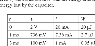
The current-voltage relationship in an element may be instantaneous but not necessarily linear. The
element is then modeled as a nonlinear resistor. An example is a filament lamp which at higher voltages
draws proportionally less current. Another important electrical device modeled as a nonlinear resistor is
a diode. A diode is a two-terminal device that, roughly speaking, conducts electric current in one
direc-tion (from anode to cathode, called forward-biased) much better than the opposite direcdirec-tion
(reverse-biased). The circuit symbol for the diode and an example of its current-voltage characteristic are shown
in Fig. 2-25. The arrow is from the anode to the cathode and indicates the forward direction (
i
> 0). A
small positive voltage at the diode’s terminal biases the diode in the forward direction and can produce
a large current. A negative voltage biases the diode in the reverse direction and produces little current
even at large voltage values. An ideal diode is a circuit model which works like a perfect switch. See
Fig. 2-26. Its (
i
,
u
)
characteristic is
υ
υ
=
≥
=
≤
0
0
0
0
when
when
i
i
The
static resistance
of a nonlinear resistor operating at (
I
,
V
)
is
R
=
V
/
I.
Its
dynamic resistance
is
r
=
∆
V
/
∆
I
which is the inverse of the slope of the current plotted versus voltage. Static and dynamic resistances both
depend on the operating point.
EXAMPLE 2.4 The current and voltage characteristic of a semiconductor diode in the forward direction is measured and recorded in the following table:
u (V) 0.5 0.6 0.65 0.66 0.67 0.68 0.69 0.70 0.71 0.72 0.73 0.74 0.75
i (mA) 2 × 10⁻⁴ 0.11 0.78 1.2 1.7 2.6 3.9 5.8 8.6 12.9 19.2 28.7 42.7
In the reverse direction (i.e., when
u
<
0),
i
=
4 × 10
−15A. Using the values given in the table, calculate
the static and dynamic resistances (
R
and
r
) of the diode when it operates at 30 mA, and find its power
consumption
p.
Fig. 2-9
From the table
EXAMPLE 2.5 The current and voltage characteristic of a tungsten filament light bulb are measured and recorded in the following table. Voltages are DC steady-state values, applied for a long enough time for the lamp to reach thermal equilibrium.
u (V) 0.5 1 1.5 2 3 3.5 4 4.5 5 5.5 6 6.5 7 7.5 8
i (mA) 4 6 8 9 11 12 13 14 15 16 17 18 18 19 20
Find the static and dynamic resistances of the filament and also the power consumption at the operating points (a) i = 10 mA; (b) i =15 mA.
again zero, and it increases linearly to 10 A at
t
=
4 ms. This pattern repeats each 2 ms. Sketch the
corresponding
u
.
Since u= Ri,the maximum voltage must be (5)(10) = 50 V. In Fig. 2-10 the plots of i and uare shown. The identical nature of the functions is evident.
2.4.
An inductance of 3.0 mH has a voltage that is described as follows: for 0 <
t
< 2 ms,
V
=
15.0 V and
for 2 <
t
< 4 ms,
V
= −
30.0 V. Obtain the corresponding current and sketch
u
Land
i
for the given
intervals.
For 0 < t < 2 ms,
i
L dt dt t
t t
= =
× = ×
∫
−∫
1 1
3 10 15 0 5 10 0
3
3 0
υ . (A)
For t= 2 ms,
i
= 10.0 A For 2 < t < 4 ms,
i
L dt dt
t t
= + +
× − −
× − × −
∫
∫
1
10 0 1
3 103 30 0
2 103 2 103
υ . .
== +
× − + ×
= −
− −
10 0 1
3 10 30 0 60 0 10 30 0
3
3
. [ . ( . )]
.
t (A)
((10×103t)(A)
See Fig. 2-12.
2.5.
A capacitance of 60.0
µ
F has a voltage described as follows: 0 <
t
<
2 ms,
u
=
25.0 × 10
3t
(V). Sketch
i
,
p
,
and
w
for the given interval and find
W
max.
Fig. 2-10
For 0 < t < 1 ms,
di
dt L
di dt L
=10×103A/s and υ = =20V When di/dt = 0, for 1 ms < t < 2ms,uL=0.
Assuming zero initial charge on the capacitor, υC =C
∫
i dt1
For 0 ≤t ≤ 1 ms,
υ
C
t
t dt t =
× −
∫
=1
5 10 4 10 10 4
0
7 2 (V) This voltage reaches a value of 10 V at 1 ms. For 1 ms < t < 2 ms, υC =(20×103)(t−10−3)+10( )V
See Fig. 2-14.
Fig. 2-14
2.8.
A single circuit element has the current and voltage functions graphed in Fig. 2-15. Determine the
element.
The element cannot be a resistor since uand i are not proportional. uis an integral of i. For 2 ms < t < 4 ms,
i ≠ 0 but uis constant (zero); hence the element cannot be a capacitor. For 0 < t < 2 ms,
di
dt = 5 10 A/s and = 15 V
3
× υ
Consequently,
L di
dt
Fig. 2-15
2.9.
Obtain the voltage
u
in the branch shown in Fig. 2-16 for (
a
)
i
2=
1 A, (
b
)
i
2= −
2
A,
(
c
)
i
2=
0 A.
Voltage uis the sum of the current-independent 10-V source and the current-dependent voltage source ux. Note that the factor 15 multiplying the control current carries the units Ω.(a)
υ=10+υx =10+15 1( )=25V (b)
υ=10+υx =10+15 2(− = −) 20V
(c)
υ=10 + 15(0) = 10 V
Fig. 2-16
2.10.
Find the power absorbed by the generalized circuit element in Fig. 2-17, for (
a
)
u
=
50 V, (
b
)
u
= −
50 V.
Fig. 2-17
2.11.
Find the power delivered by the sources in the circuit of Fig. 2-18.
i =20−50 = −
3 10 A The powers absorbed by the sources are:
pa = −υai= −(20)(−10)=200 W
p i
b=υb =(50)(−10)= −500 W
Since power delivered is the negative of power absorbed, source ub delivers 500 W and source ua absorbs 200 W. The power in the two resistors is 300 W.
2.12.
A 25.0-
Ω
resistance has a voltage
u
=
150.0 sin 377
t
(V). Find the power
p
and the average power
p
avgover one cycle.
i=υ/R=6 0. sin377t (A) p=υi=900 0. sin2377t(W)
The end of one period of the voltage and current functions occurs at 377t =2p. For Pavg, the integration is taken over one-half cycle, 377t= p. Thus,
Pavg= 1
∫
900 0 2 377t d 377t =450 0(W) 0π π
. sin ( ) ( ) .
2.13.
Find the voltage across the 10.0-
Ω
resistor in Fig. 2-19 if the control current
i
xin the dependent source
is (
a
)
2 A
and (
b
)
−
1 A.
i i iR i
i
x R x
x R
4 4 (V)
2 A
= − = = −
= =
. ; . .
;
0 40 0 40 0
4 υ
υ 00 0 80 0
.
; .
V
1 A V
ix = − υR = −
Fig. 2-18
SUPPLEMENTARY PROBLEMS
2.14. A resistor has a voltage of V= 1.5 mV. Obtain the current if the power absorbed is (a) 27.75 nW and (b) 1.20 µW.
Ans. 18.5 µA, 0.8 mA
2.15. A resistance of 5.0 Ωhas a current i =5.0 × 10³t (A) in the interval 0 ≤t ≤ 2 ms. Obtain the instantaneous and average powers. Ans. 125.0t2 (W), 167.0 (W)
2.16. Current i enters a generalized circuit element at the positive terminal and the voltage across the element is 3.91 V. If the power absorbed is −25.0 mW, obtain the current. Ans. −6.4 mA
2.17. Determine the single circuit element for which the current and voltage in the interval 0 ≤ 103 t ≤ pare given by
i =2.0 sin 103 t (mA) and u=5.0 cos 103 t (mV). Ans. An inductance of 2.5 mH
2.18. An inductance of 4.0 mH has a voltage u=2 0. e−103t (V). Obtain the maximum stored energy. At t =0, the current is zero. Ans. 0.5 mW
2.19. A capacitance of 2.0 µF with an initial charge Q0 is switched into a series circuit consisting of a 10.0-Ω resistance. Find Q0 if the energy dissipated in the resistance is 3.6 mJ. Ans. 120.0 µC
2.20. Given that a capacitance of C farads has a current i =(Vm/R)e−t/(Rc) (A), show that the maximum storedenergy is 1
2 2
CVm. Assume the initial charge is zero.
2.21. The current after t =0 in a single circuit element is as shown in Fig. 2-20. Find the voltage across the element at t =6.5 µs, if the element is (a)a resistor with resistance of 10 kΩ, (b)an inductor with inductance of 15 mH, (c)a0.3 nF capacitor with Q(0) = 0.
Ans. (a)25 V; (b) −75 V; (c)81.3 V
Fig. 2-20
Fig. 2-21
2.22. The 20.0-µF capacitor in the circuit shown in Fig. 2-21 has a voltage for t > 0, u=100.0e−t/0.015 (V). Obtain the energy function that accompanies the discharge of the capacitor and compare the total energy to that which is absorbed by the 750-Ω resistor. Ans. 0.10 (1 −e−t/0.0075) (J)
2.23 Find the current i in the circuit shown in Fig. 2-22, if the control u2of the dependent voltage source has the value (a)4 V, (b)5 V, (c)10 V. Ans. (a)1 A; (b)0 A; (c) −5 A
2.24 In the circuit shown in Fig. 2-23, find the current, i,given (a) i1=2A, i2=0; (b) i1= −1A, i2= 4 A;(c) i1= i2= 1 A.
2.25. A 1-µF capacitor with an initial charge of 10−4 C is connected to a resistor R at t =0. Assume discharge current during 0 < t < 1 ms is constant. Approximate the capacitor voltage drop at t =1 ms for
(a)R = 1 MΩ;(b)R = 100 kΩ;(c)R =10 kΩ. Hint: Compute the charge lost during the 1-ms period.
Ans. (a)0.1 V; (b)1 V; (b)10 V
2.26. The actual discharge current in Problem 2.25 is i=(100/R e) −106t R/ A. Find the capacitor voltage drop at 1 ms after connection to the resistor for (a) R = 1 MΩ; (b) R = 100 kΩ;(c)R = 10 kΩ.
Ans. (a)0.1 V; (b)1 V; (c)9.52 V
2.27. A 10-µF capacitor discharges in an element such that its voltage is u=2e−1000t.Find the current and power delivered by the capacitor as functions of time.
Ans. i =20e−1000t mA, p = vi =40e−1000t mJ
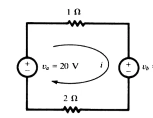
2.28. Find voltage u, current i, and energy W in the capacitor of Problem 2.27 at time t =0, 1, 3, 5, and 10 ms. By integrating the power delivered by the capacitor, show that the energy dissipated in the element during the interval from 0 to t is equal to the energy lost by the capacitor.
Ans.
t u i W
0 2 V 20 mA 20 µJ
1 ms 736 mV 7.36 mA 2.7 µJ 3 ms 100 mV 1 mA 0.05 µJ 5 ms 13.5 mV 135 µA ≈ 0.001 µJ 10 ms 91 µV 0.91 µA ≈ 0 J
2.29. The current delivered by a current source is increased linearly from zero to 10 A in 1 ms time and then is decreased linearly back to zero in 2 ms. The source feeds a 3-kΩresistor in series with a 2-H inductor (see Fig. 2-24). (a)Find the energy dissipated in the resistor during the rise time (W1)and the fall time (W2). (b)Find the energy delivered to the inductor during the above two intervals. (c)Find the energy delivered by the current source to the series RL combination during the preceding two intervals. Note:Series elements have the same current. The voltage drop across their combination is the sum of their individual voltages.
Ans. (a) W1=100, W2=200; (b) W1=200, W2= −200; (c) W1=300, W2=0 (All in joules)
Fig. 2-22 Fig. 2-23
2.30. The voltage of a 5-µF capacitor is increased linearly from zero to 10 V in 1 ms time and is then kept at that level. Find the current. Find the total energy delivered to the capacitor and verify that delivered energy is equal to the energy stored in the capacitor.
Ans. i =50 mA during 0 < t < 1 ms and is zero elsewhere, W = 250 µJ.
2.31. A 10-µF capacitor is charged to 2 V. A path is established between its terminals which draws a constant current of I0. (a)For I0= 1 mA, how long does it take to reduce the capacitor voltage to 5 percent of its initial value? (b)For what value of I0does the capacitor voltage remain above 90 percent of its initial value after passage of 24 hours? Ans. (a)19 ms, (b)23.15 pA
2.32. Energy gained (or lost) by an electric charge q traveling in an electric field is q u, where uis the electric potential gained (or lost). In a capacitor with charge Q and terminal voltage V, let all charges go from one plate to the other. By way of computation, show that the total energy W gained (or lost) is not QV but QV/2and explain why. Also note that QV/2is equal to the initial energy content of the capacitor.
Ans. W=
∫
q dtυ = Q V−0 =QV = CV2 12
2 2
/ .The apparent discrepancy is explained by the following. The starting voltage between the two plates is V. As the charges migrate from one plate of the capacitor to the other plate, the voltage between the two plates drops and becomes zero when all charges have moved. The average of the voltage during the migration process is V/2and, therefore, the total energy is QV/2.
2.33. Lightning I. The time profile of the discharge current in a typical cloud-to-ground lightning strike is modeled by a triangle. The surge takes 1 µs to reach the peak value of 100 kA and then is reduced to zero in 99 µS. (a)Find the electric charge Q discharged. (b)If the cloud-to-ground voltage before the discharge is 400 MV, find the total energy W released and the average power P during the discharge. (c) If during the storm there is an average of 18 such lightning strikes per hour, find the average power released in 1 hour.
Ans. (a)Q = 5C; (b)W = 109 J, P = 1013 W; (c) 5 MW
2.34. Lightning II. Find the cloud-to-ground capacitance in Problem 2.33 just before the lightning strike.
Ans. 12.5 µF
2.35. Lightning III. The current in a cloud-to-ground lightning strike starts at 200 kA and diminishes linearly to zero in 100 µs. Find the energy released W and the capacitance of the cloud to ground C if the voltage before the discharge is (a) 100 MV; (b)500 MV.
Ans. (a) W = 5 × 10⁸ J, C = 0.1 µF; (b)W = 25 × 108 J, C = 20 nF
2.36. The semiconductor diode of Example 2.4 is placed in the circuit of Fig. 2-25. Find the current for (a) Vs=1 V, (b) Vs= −1 V. Ans. (a)14 mA; (b)0 A
2.37. The diode in the circuit of Fig. 2-26 is ideal. The inductor draws 100 mA from the voltage source. A 2-µF capacitor with zero initial charge is also connected in parallel with the inductor through an ideal diode such that the diode is reversed biased (i.e., it blocks charging of the capacitor). The switch s suddenly disconnects with the rest of the circuit, forcing the inductor current to pass through the diode and establishing 200 V at the capacitor’s terminals. Find the value of the inductor. Ans. L = 8 H
Fig. 2-26
2.38. Compute the static and dynamic resistances of the diode of Example 2.4 at the operating point u= 0.66 V.
Ans. R≈ r
× = ≈
− − −
0 66
1 2 10 550
0 67 0 65 1 7 0 78 3
. .
. .
( . . ) Ω and
××10−3 =21 7. Ω
2.39. The diode of Example 2.4 operates within the range 10 mA < i < 20 mA. Within that range, approximate its terminal characteristic by a straight line i =au+b, by specifying aand b.
Ans. i =630 u −4407 mA, where uis in V.
2.40. The diode of Example 2.4 operates within the range of 20 mA < i < 40 mA. Within that range, approximate its terminal characteristic by a straight line connecting the two operating limits.
Ans. i =993.33 u −702.3 mA, where uis in V.
2.41. Within the operating range of 20 mA < i < 40 mA, model the diode of Example 2.4 by a resistor R in series with a voltage source V such that the model matches exactly with the diode performance at 0.72 V and 0.75 V. Find R and V.
24
Circuit
Laws
3.1 Introduction
An electric circuit or network consists of a number of interconnected single circuit elements of the type
described in Chapter 2. The circuit will generally contain at least one voltage or current source. The
arrange-ment of elearrange-ments results in a new set of constraints between the currents and voltages. These new constraints
and their corresponding equations, added to the current-voltage relationships of the individual elements,
provide the solution of the network.
The underlying purpose of defining the individual elements, connecting them in a network, and solving
the equations is to analyze the performance of such electrical devices as motors, generators, transformers,
electrical transducers, and a host of electronic devices. The solution generally answers necessary questions
about the operation of the device under conditions applied by a source of energy.
3.2 Kirchhoff’s Voltage Law
For any closed path in a network,
Kirchhoff ’s voltage law
(KVL) states that the algebraic sum of the
volt-ages is zero. Some of the voltvolt-ages will be sources, while others will result from current in passive elements
creating a voltage, which is sometimes referred to as a
voltage drop.
The law applies equally well to circuits
driven by constant sources, DC, time variable sources,
u
(
t
) and
i
(
t
), and to circuits driven by sources which
will be introduced in Chapter 9. The mesh current method of circuit analysis introduced in Section 4.2 is
based on KVL.
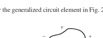
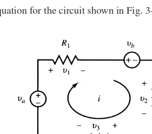
EXAMPLE 3.1 Write the KVL equation for the circuit shown in Fig. 3-1.
Fig. 3-1
Starting at the lower left corner of the circuit, for the current direction as shown, we have −
−
υ υ υ υ υ
υ υ
a b
a iR b iR iR
+ + + + = 0
+ + + +
1 2 3
2 3
1 = 0
3.3 Kirchhoff’s Current Law
The connection of two or more circuit elements creates a junction called a
node
. The junction between two
elements is called a
simple node
and no division of current results. The junction of three or more elements
is called a
principal node
, and here current division does take place.
Kirchhoff ’s current law
(KCL) states
that the algebraic sum of the currents at a node is zero. It may be stated alternatively that the sum of the
currents entering a node is equal to the sum of the currents leaving that node. The node voltage method of
circuit analysis introduced in Section 4.3 is based on equations written at the principal nodes of a network by
applying KCL. The basis for the law is the conservation of electric charge.
EXAMPLE 3.2 Write the KCL equation for the principal node shown in Fig. 3-2.
i i i i i
i i i i i
1 2 3 4 5
1 3 2 4 5
0 − + − − =
+ = + +
Fig. 3-2
Fig. 3-3