123
Dan Wang
Zhu Han
Sublinear
Algorithms
for Big Data
Applications
Series Editors
Stan Zdonik Shashi Shekhar Jonathan Katz Xindong Wu Lakhmi C. Jain David Padua
Xuemin (Sherman) Shen Borko Furht
VS Subrahmanian Martial Hebert Katsushi Ikeuchi Bruno Siciliano Sushil Jajodia Newton Lee
More information about this series athttp://www.springer.com/series/10028
Sublinear Algorithms
for Big Data Applications
123
Department of Computing
The Hong Kong Polytechnic University Kowloon, Hong Kong, SAR
Department of Engineering University of Houston Houston, TX, USA
ISSN 2191-5768 ISSN 2191-5776 (electronic)
SpringerBriefs in Computer Science
ISBN 978-3-319-20447-5 ISBN 978-3-319-20448-2 (eBook) DOI 10.1007/978-3-319-20448-2
Library of Congress Control Number: 2015943617 Springer Cham Heidelberg New York Dordrecht London © The Author(s) 2015
This work is subject to copyright. All rights are reserved by the Publisher, whether the whole or part of the material is concerned, specifically the rights of translation, reprinting, reuse of illustrations, recitation, broadcasting, reproduction on microfilms or in any other physical way, and transmission or information storage and retrieval, electronic adaptation, computer software, or by similar or dissimilar methodology now known or hereafter developed.
The use of general descriptive names, registered names, trademarks, service marks, etc. in this publication does not imply, even in the absence of a specific statement, that such names are exempt from the relevant protective laws and regulations and therefore free for general use.
The publisher, the authors and the editors are safe to assume that the advice and information in this book are believed to be true and accurate at the date of publication. Neither the publisher nor the authors or the editors give a warranty, express or implied, with respect to the material contained herein or for any errors or omissions that may have been made.
Printed on acid-free paper
Springer International Publishing AG Switzerland is part of Springer Science+Business Media (www. springer.com)
Dedicate to my family, Zhu Han
In recent years, we see a tremendously increasing amount of data. A fundamental challenge is how these data can be processed efficiently and effectively. On one hand, many applications are looking for solid foundations; and on the other hand, many theories may find new meanings. In this book, we study one specific advancement in theoretical computer science, the sublinear algorithms and how they can be used to solve big data application problems. Sublinear algorithms, as what the name shows, solve problems using less than linear time or space as against to the input size, with provable theoretical bounds. Sublinear algorithms were initially derived from approximation algorithms in the context of randomization. While the spirit of sublinear algorithms fit for big data application, the research of sublinear algorithms is often restricted within theoretical computer sciences. Wide application of sublinear algorithms, especially in the form of current big data applications, is still in its infancy. In this book, we take a step towards bridging such gap. We first present the foundation of sublinear algorithms. This includes the key ingredients and the common techniques for deriving the sublinear algorithm bounds. We then present how to apply sublinear algorithms to three big data application domains, namely, wireless sensor networks, big data processing in MapReduce, and smart grids. We show how problems are formalized, solved, and evaluated, such that the research results of sublinear algorithms from the theoretical computer sciences can be linked with real-world problems.
We would like to thank Prof. Sherman Shen for his great help in publishing this book. This book is also supported by US NSF CMMI-1434789, CNS-1443917, ECCS-1405121, CNS-1265268, and CNS- 0953377, National Natural Science Foundation of China (No. 61272464), and RGC/GRF PolyU 5264/13E.
Kowloon, Hong Kong Dan Wang
Houston, TX, USA Zhu Han
vii
1 Introduction . . . 1
1.1 Big Data: The New Frontier. . . 1
1.2 Sublinear Algorithms. . . 4
1.3 Book Organization. . . 6
References. . . 7
2 Basics for Sublinear Algorithms . . . 9
2.1 Introduction . . . 9
2.2 Foundations . . . 10
2.2.1 Approximation and Randomization. . . 10
2.2.2 Inequalities and Bounds. . . 11
2.2.3 Classification of Sublinear Algorithms. . . 12
2.3 Examples. . . 13
2.3.1 Estimating the User Percentage: The Very First Example. . . 13
2.3.2 Finding Distinct Elements. . . 14
2.3.3 Two-Cat Problem. . . 18
2.4 Summary and Discussions. . . 20
References. . . 21
3 Application on Wireless Sensor Networks . . . 23
3.1 Introduction . . . 23
3.1.1 Background and Related Work. . . 24
3.1.2 Chapter Outline. . . 26
3.2 System Architecture . . . 26
3.2.1 Preliminaries. . . 26
3.2.2 Network Construction. . . 26
3.2.3 Specifying the Structure of the Layers. . . 28
3.2.4 Data Collection and Aggregation. . . 28
3.3 Evaluation of the Accuracy and the Number of Sensors Queried. . . 29
3.3.1 MAX and MIN Queries. . . 29
3.3.2 QUANTILE Queries. . . 30
ix
6 Concluding Remarks . . . 83
6.1 Summary of the Book. . . 83
Introduction
1.1
Big Data: The New Frontier
In February 2010, National Centers for Disease Control and Prevention (CDC) identified an outbreak of flu in the mid-Atlantic regions of the United States. However, 2 weeks earlier, Google Flu Trends [1] had already predicted such an outbreak. By no means does Google have more expertise in the medical domain than the CDC. However, Google was able to predict the outbreak early because it uses big data analytics. Google establishes an association between outbreaks of flu and user queries, e.g., on throat pain, fever, and so on. The association is then used to predict the flu outbreak events. Intuitively, an association means that if event A (e.g., a certain combination of queries) happens, event B (e.g., a flu outbreak) will happen (e.g., with high probability). One important feature of such analytics is that the association can only be established when the data is big. When the data is small, such as a combination of a few user queries, it may not expose any connection with a flu outbreak. Google applied millions of models to the huge number of queries that it has. The aforementioned prediction of flue by Google is an early example of the power of big data analytics, and the impact of which has been profound.
The number of successful big data applications is increasing. For example, Amazon uses massive historical shipment tracking data to recommend goods to targeted customers. Indeed such “Target Marketing” has been adopted and is being carried out by all business sectors that have penetrated all aspects of our life. We see personalized recommendations from the web pages we commonly visit, from the social network applications we use daily, and from the online game stores we frequently access. In smart cities, data on people, the environment, and the operational components of the city are collected and analyzed (see Fig.1.1). More specifically, data on traffic and air quality reports are used to determine the causes of heavy air pollution [3], and the huge amount of data on bird migration paths are analyzed to predict H5N1 bird flu [4]. In the area of B2B, there are startup companies (e.g., MoleMart, MolBase) that analyze huge amount
© The Author(s) 2015
D. Wang, Z. Han,Sublinear Algorithms for Big Data Applications, SpringerBriefs in Computer Science, DOI 10.1007/978-3-319-20448-2_1
Fig. 1.1 Smart City, a big vision of the future where people, environment, and city operational components are in harmony. One key to achieve this is big data analytics, where data of people, environment and city operational components are collected and analyzed. The data variety is diverse, the volume is big, the collection velocity can be high, and the veracity may be problematic; yet handling these
appropriately, the value can be significant
of data on pharmaceutical, biological, and chemical related industries. Accurate connections between buyers and vendors are established and the risk to companies of overstocking or understocking is reduced. This has lead to cost reductions of more than ten times compared to current B2B intermediaries.
The expectations for the future are even greater. Today, scientists, engineers, educators, citizens, and decision-makers have unprecedented amounts and types of data available to them. Data come from many disparate sources, including scientific instruments, medical devices, telescopes, microscopes, and satellites; digital media including text, video, audio, email, weblogs, twitter feeds, image collections, click streams, and financial transactions; dynamic sensors, social, and other types of networks; scientific simulations, models, and surveys; or from computational analysis of observational data. Data can be temporal, spatial, or dynamic; and structured or unstructured. Information and knowledge derived from data can differ in representation, complexity, granularity, context, provenance, reliability, trustworthiness, and scope. Data can also differ in the rate at which they are generated and accessed.
Previous studies often focused on handling complexity in terms of computation-intensive operations. The focus has now switched to handling complexity in terms of data-intensive operations. In this respect, studies are carried out on every front. Notably, there are studies from the system perspective. These studies address the handling of big data at the processor level, at the physical machine level, at the cloud virtualization level, and so on. There are studies on data networking for big data communications and transmissions. There are also studies on databases to handle fast indexing, searches, and query processing. In the system perspective, the objective is to ensure efficient data processing performance, with trade-offs on load balancing, fairness, accuracy, outliers, reliability, heterogeneity, service level agreement guarantees, and so on.
Nevertheless, with the aforementioned real world applications as the demand, and the advances of the storage, system, networking and database support as the supply, their direct marriage may still result in unacceptable performance. As an example, smart sensing devices, cameras, and meters are now widely deployed in urban areas. Frequent checking needs to be made of certain properties of these sensor data. The data is often big enough that even process each piece of the data just once can consume a great deal of time. Studies from the system perspective usually do not provide an answer to the issue of which data should be processed (or given higher priority in processing) and which data may be omitted (or given a lower priority in processing). Novel algorithms, optimizations, and learning techniques are thus urgently needed in data analytics to wisely manage the data.
From a broader perspective, data and the knowledge discovery process involve a cycle of analyzing data, generating a hypothesis, designing and executing new experiments, testing the hypothesis, and refining the theory. Realizing the trans-formative potential of big data requires many challenges in the management of data and knowledge to be addressed, computational methods for data analysis to be devised, and many aspects of data-enabled discovery processes to be automated. Combinations of computational, mathematical, and statistical techniques, method-ologies and theories are needed to enable these advances to be made. There have been many new advances in theories and methodologies on data analytics, such as sparse optimization, tensor optimization, deep neural networks (DNN), and so on. In applying these theories and methodologies to the applications, specific application requirements can be taken into consideration, thus wisely reducing, shaping, and organizing the data. Therefore, the final processing of data in the system can be significantly more efficient than if the application data had been processed using a brute force approach.
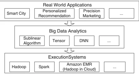
An overall picture of the big data processing is given in Fig.1.2. At the top are real world applications, where specific applications are designed and the data are collected. Appropriated algorithms, theories, or methodologies are then applied to assist knowledge discovery or data management. Finally, the data are stored and processed in the execution systems, such as Hadoop, Spark, and others.
ExecutionSystems Big Data Analytics Real World Applications
Personalized Recommendation
Smart City Precision
Marketing
Hadoop
...
Sublinear
Algorithm Tensor DNN ...
Spark Amazon EMR
(Hadoop in Cloud) ...
Fig. 1.2 A overall picture: from real world applications to big data analytics to execution systems
performance of the sublinear algorithms, in terms of time, storage space, and so on, is less than linear as against the amount of input data. More importantly, sublinear algorithms provide guarantees of accuracy of the output from the algorithms.
1.2
Sublinear Algorithms
Research on sublinear algorithms began some time ago. Sublinear algorithms were initially developed in the theoretical computer science community. The sublinear algorithm is one further classification of the approximation algorithm. Its study involves the long-debated issue of the trade-off between algorithm processing time and algorithm output quality.
In a conventional approximation algorithm, the algorithm can output an approxi-mate result that deviates from the optimal result (within a bound), yet the algorithm processing time can become faster. One hidden implication of the design is that the approximate result is 100 % guaranteed within this bound. In a sublinear algorithm, such an implication is relaxed. More specifically, a sublinear algorithm outputs an approximate result that deviates from the optimal result (within a bound) for a (usually) majority of the time. As a concrete example, a sublinear algorithm usually says that the output of the algorithm differs from the optimal solution by at most 0.1 (the bound) at least 95 % of the time (the confidence).
This transition is important. From the theoretical research point of view, a new category is developed. From the practical point of view, sublinear algorithms provide two controlling parameters for the user in making trade-offs, while approx-imation algorithms have only one controlling parameter.
from stochastic techniques, which analyze the mean and variance of a system in a steady state. For example, a typical queuing theory result is that the expected waiting time is 100 s.
In the theoretical computer sciences in the past few years, there have been many studies on sublinear algorithms. Sublinear algorithms have been developed for many classic computer science problems, such as finding the most frequently element, finding distinct elements, etc.; and for graph problems, such as finding the minimum spanning tree, etc.; and for geometry problems, such as finding the intersection of two polygons, etc. Sublinear algorithms can be broadly classified into sublinear time algorithms, sublinear space algorithms, and sublinear communication algorithms, where the amount of time, storage space, or communications needed iso.N/withN
as the input size.
Sublinear algorithms are a good match of big data analytics. Decisions can be drawn by only looking at a subset of the data. In particular, sublinear algorithms are suitable for situations, where the total amount of data is so massive that even linear processing time is not affordable. Sublinear algorithms are also suitable for situations, where some initial investigations need to be made before looking into the full data set. In many situations, the data are massive but it is not known whether the value of the data is big or not. As such, sublinear algorithms can serve to give an initial “peek” of the data before more a in-depth analysis is carried out. For example, in bioinformatics, we need to test whether certain DNA sequences are periodic. Sublinear algorithms, when appropriately designed to test periodicity in data sequences, can be applied to rule out useless data.
While there have been decent advances in the past few years in research on sublinear algorithms, to date, the study of sublinear algorithms has often been restricted to the theoretical computer sciences. There have been some applications. For example, in databases, where sublinear algorithms are used for the efficient query processing such as top-k queries; in bioinformatics, sublinear algorithms are used for testing whether a DNA sequence shows periodicity; and in networking, sublinear algorithms are used for testing whether two network traffic flows are close in distribution. Nevertheless, sublinear algorithms have yet to be applied, especially in the form of current big data applications. Tutorials on sublinear algorithms from the theoretical point of view, with a collection of different sublinear algorithms, aimed at better approximation bounds, are particularly abundant [2]. Yet there are far fewer applications of sublinear algorithms, aimed at application background scenarios, problem formulations, and evaluations of parameters. This book is not a collection of sublinear algorithms; rather, the focus is on the application of sublinear algorithms.
behavior analysis using metering data from smart grids. We show how the problem should be formalized, solved, and evaluated, so that the sublinear algorithms can be used to help solve real-world problems.
1.3
Book Organization
The purpose of this book is to give a snapshot of sublinear algorithms and their applications. Different from other writings on sublinear algorithms, we focus on learning the basic ideas of sublinear algorithms, rather than on presenting a comprehensive survey of the sublinear algorithms found in literature. We also target the issue of when and how to apply sublinear algorithms to applications. This includes learning in what situations the sublinear algorithms may fit into certain scenarios, how we may combine multiple sublinear algorithms to solve a problem, how to develop sublinear algorithms with additional statistical information, what structures are needed to support sublinear algorithms, and how we may extend existing sublinear algorithms to fit into applications. The remaining five chapters of the book are organized as follows.
In Chap.2, we present the basic concepts of the sublinear algorithm. We first present the main thread of theoretical research on sublinear algorithms and discuss how sublinear algorithms are related to other theoretical developments in the computing sciences, in particular, approximation and randomization. We then present preliminary mathematical techniques on inequalities and bounds. We then give three examples. The first is on estimating the percentage of households among a group of people. This is an illustration of the direct application of inequalities and bounds to derive a sublinear algorithm. The second is on finding distinct elements. This is a classical sublinear algorithm. The example involves some key insights and techniques in the development of sublinear algorithms. The third is a two cat problem where we develop an algorithm that is sublinear, but which does not fall into standard sublinear algorithm format. The example provides some additional thoughts on the wide spectrum of sublinear algorithms.
big data processing, MapReduce, and a data skew problem within the MapReduce framework. We show that the overall problem is a load balancing problem, and we formulate the problem. The problem calls for the use of an online algorithm. We first develop a straightforward online algorithm and prove that it is 2-competitive. We then show that by sampling a subset of the data, we can make wiser decisions. We develop an algorithm and analyze the amount of data that we need to “peek” before we can make theoretical guaranteed decisions. Intrinsically, this is a sublinear algorithm. In this application, the sublinear algorithm is not the solution for the entire problem space. We show that the sublinear algorithm assists in solving a data skew problem so that the overall solution is a more accurate one.
In Chap.5, we present an application of sublinear algorithms for a behavior analysis using metering data from a smart grid. Smart meters are now widely deployed where it is possible to collect fine-grained data on the electricity usage of users. One objective is to conduct a classification of the users based on data of their electricity use. We choose to use the electricity usage distribution as the criterion for classification, as it captures more information on the behavior of a user. Such classification can be used for customized differentiated pricing, energy conservation, and so on. In this chapter, we first present a trace analysis on the smart metering data that we collected, which were recorded for 2.2 million households in the great Houston area. For each user, we recorded the electricity used every 15 min. Clearly, we face a big data problem. We develop a sublinear algorithm, where we apply an existing sublinear algorithm that was developed in the literature as a sub-function. Finally, we present differentiated services for a utility company. This shows a possible case of the use of user classifications to maximize the revenue of the utility company.
In Chap.6, we present some experiences in the development of sublinear algo-rithms and a summary of the book. We discuss the fitted scenarios and limitations of sublinear algorithms as well as the opportunities and challenges to the use of sublinear algorithms. We conclude that there is an urgent need to apply the sublinear algorithms developed in the theoretical computer sciences to real-world problems.
References
1. Google Flu Prediction, available athttp://www.google.org/flutrends/.
2. R. Rubinfeld, Sublinear Algorithm Surveys, available at http://people.csail.mit.edu/ronitt/ sublinear.html.
3. Y. Zheng, F. Liu, and H. P. Hsieh, “U-Air: When Urban Air Quality Inference meets big Data”, inProc. ACM SIGKDD’13, 2013.
Basics for Sublinear Algorithms
2.1
Introduction
In this chapter, we study the theoretical foundations of sublinear algorithms. We discuss the foundations of approximation and randomization and show the history of the development of sublinear algorithms in the theoretical research line. Intrinsically, sublinear algorithms can be considered as one branch of approximation algorithms with confidence guarantees. A sublinear algorithm says that the accuracy of the algorithm output will not deviate from an error bound and there is high confidence that the error bound will be satisfied. More rigidly, a sublinear algorithm is commonly written as.1C; ı/-approximation in a mathematical form. Hereis commonly called anaccuracy parameter andı is commonly called aconfidence parameter. This accuracy parameter is the same to the approximate factor in approximation algorithms. This confidence parameter is the key trade-off where the complexity of the algorithm can reduce to sublinear. We will rigidly define these parameters in this chapter.
Then we present some inequalities, such as Chernoff inequality and Hoeffding inequality, which are commonly used to derive the bounds for the sublinear algorithms. We further present the classification of sublinear algorithms, namely sublinear algorithms in time, sublinear algorithms in space, and sublinear algorithms in communication.
Three examples will be instanced in this chapter to illustrate how sublinear algorithms (in particular, the bounds), which are developed from the theoretical point of view. The first example is a straightforward application of Hoeffding inequality. The second one is a classic sublinear algorithm to find distinct elements. In the third example, we show a sublinear algorithm that does not belong to the standard form of.; ı/ approximation. This can further broaden the view on sublinear algorithms.
© The Author(s) 2015
D. Wang, Z. Han,Sublinear Algorithms for Big Data Applications, SpringerBriefs in Computer Science, DOI 10.1007/978-3-319-20448-2_2
9
2.2
Foundations
2.2.1
Approximation and Randomization
We start by considering algorithms. An algorithm is a step-by-step calculating procedure for solving a problem and outputting a result. In common sense, an algorithm tries to output an optimal result. When evaluating an algorithm, an important metric is its complexity. There are different complexity classes. Two most important classes are P and NP. The problems in P are those that can be solved in polynomial times and the problems in NP are those that must be solved in super-polynomial times. Using today’s computing architecture, running super-polynomial time algorithms is considered tolerable within their finishing times.
To handle the problems in NP, a development from theoretical computer science is to introduce a trade-off where we sacrifice the optimality of the output result so as to reduce the algorithm complexity. More specifically, we do not need to achieve the exact optimal solution; yet it is acceptable if we know that the output is close to the optimal solution. This is calledapproximation. Approximation can be rigidly defined. We show one example on a.1C/-approximation.
LetY be a problem space andf.Y/be the procedure to output a result. We call an algorithm a.1C/-approximation if this algorithm returnsOf.Y/instead of the optimal solutionf.Y/, and
jOf.Y/ f.Y/j f.Y/
Two comments have been made here. First, there can be other approximation criteria beyond.1C/-approximation. Second, approximation, though introduced mostly for NP problems, is not restricted to NP problems. One can design an approximation algorithm for the problems in P to further reduce the algorithm complexity as well.
A hidden assumption of approximation is that an approximation algorithm requests that its output is always, i.e., 100 %, within an factor of the optimal solution. A further development from theoretical computer sciences is to introduce another trade-off between optimality and algorithm complexity; that is, it is acceptable that the algorithm output is close to the optimal most of the times. For example, 95 % of time, the output result is close to the optimal result. Such probabilistic nature requires an introduction ofrandomization. We call an algorithm a .1C; ı/-approximation if this algorithm returnsfO.Y/instead of the optimal solutionf.Y/, and
PrŒjOf.Y/ f.Y/j f.Y/1 ı
Discussion: We have seen two steps in theoretical computer sciences in trading-off optimality and complexity. Such trade-trading-off does not immediately lead to an algorithm that is sublinear to its input, i.e.,.1C; ı/-approximation is not nec-essarily sublinear. Nevertheless, these provide better categorization on algorithms. In particular, the second advancement in randomization makes a sublinear algorithm possible. As discussed in the introduction, processing the full data may not be tolerable in the big data era. As a matter of fact, practitioners have already designed many schemes using only partial data. These designs may be ad hoc in nature and may not have rigid proofs in their quality. Thus, from a quality-control’s point of view, the.1 C; ı/-approximation brings to the practitioners a rigid theoretical evaluation benchmark when evaluating their designs.
2.2.2
Inequalities and Bounds
One may recall that the above formulas are similar to those inequalities in probability theory. The difference is that the above formulas and bounds are used on algorithms and in probability theory, the formulas and bounds are used on variables. In reality, many developments of sublinear algorithms heavily apply probability inequalities. Therefore, we state a few mostly used inequalities here and we will use examples to show how they will be applied to sublinear algorithm development.
Markov inequality: For a nonnegative random variable X, and anya > 0, we have
PrŒXa EŒX
a
Markov inequality is a loose bound. The good thing is that Markov inequality requires no assumptions on the random variableX.
Chernoff inequality: For independent random Bernoulli variables Xi, let XDPXi. For any, we have
PrŒX.1 /EŒXe EŒX22
Chernoff bound is tighter. Note, however, that it requires the random variables to be independent.
Chernoff inequality has many variations. Practitioners may often encounter a problem of computingPrŒX kwherekis a parameter of real world importance. Especially, one may want to linkkwithı. For example, given that the expectation ofXis known, how can thekbe determined so that the probabilityPrŒX kis at least1 ı. Such linkage betweenkandıcan be derived from Chernoff inequality as follows:
PrŒXkDPrŒX k
EŒXEŒX
Let1 D k
EŒX and with Chernoff inequality we have:
PrŒXke
EŒX.1 EŒkX/2
2 Then, to linkıandk, we have
PrŒXke
EŒX.1 EŒkX/2
2 1 ı
Note that the last inequality provides a connection betweenkandı.
Chebyshev inequality: For anyXwithEŒXDandVarŒXD2, and for any
a> 0,
PrŒjX j a 1
a2
Hoeffding inequality: Assume we have k random identical and independent variablesXi, for any, we have
PrŒjX EŒXj e 22k
Hoeffding inequality is commonly used to bound the deviation from the mean.
2.2.3
Classification of Sublinear Algorithms
The most common classification of sublinear algorithms is to see whether a sublinear algorithm useso.N/in space oro.N/in time oro.N/in communication, whereNis the input size. Respectively, they are called sublinear algorithms in time, sublinear algorithms in space or sublinear algorithms in communication.
data is coming in a streaming fashion. In other words, the data comes in an online fashion and it is possible to read each piece of data as time progresses. Yet the challenge is that it is impossible to store all these data in storage because the data is too large. The result of the algorithm is usingo.N/space, whereNis the storage space. Such category is also commonly called as data stream algorithms. Sublinear algorithms in communication mean that the data is too large to be stored in a single machine and one needs to make decision through collaboration between machines. It is only possible to use o.N/communications, whereN is the total number of communications.
There are algorithms that do not fall into the..1C/; ı/-approximation category. A typical example is when there needs of a balance between the resources such as storage, communications, and time. Therefore, algorithms can be developed where the contribution of each type of resources is sublinear; and they collectively achieve the task. One example of such kind can be found from a sensor data collection application in [2]. In this example, a data collection task is achieved with a sublinear sacrifice of storage and a sublinear sacrifice of communication.
In this chapter, we will present a few examples. The first one is a simple example on estimating percentage. We show how the bound of a sublinear algorithm can be derived using inequalities. This is a sublinear algorithm in time. Then we discuss a classic sublinear algorithm to find distinct elements. The idea is to see how we can go beyond simple sampling and quantify an idea and develop quantitative bounds. In this example, we also show the median trick, a classic trick in managingı. This is a sublinear algorithm in space. Finally, we discuss a two-cat problem, where its intuition is applied in [2]. This divides two resources and collectively achieves a task.
2.3
Examples
2.3.1
Estimating the User Percentage: The Very First Example
We start from a simple example. Assume that there is a group of people, who can be classified into different categories. One category is the housewife. The question is that we want to know the percentage of the housewife in this group, but the group is too big to examine every person. A simple way is to sample a subset of people and see how many of these people in it belong to the housewife group. This is where the question arise: how many samples are enough?
Theorem 2.1. Given; ı, to guarantee that we have a probability of1 ısuccess that the percentage (e.g., of housewife) will not deviate from˛for more than, the number of users we need to sample must be at least log22ı.
We first conduct some analyses. LetNbe the total number of users and letmbe the number of users we sample. LetYibe an indicator random variable where
YiD
1;housewife
0;otherwise
We assume thatYiare independent, i.e., Alice belongs to the housewife group is
independent of whether Mary belongs to housewife or not.
Let Y D PNiD1Yi. By definition, we have ˛ D N1EŒY. Since Yi are all
independent,EŒYi D ˛. LetX D P m
iD1Yi. LetX D m1X. The next lemma says
that the expectationXof the sampled set is the same as the expectation of the whole set.
Lemma 2.1. EŒXD˛.
Proof. EŒXD m1EŒPm1 YiD m1 m˛D˛. ut
We next proof Theorem2.1.
Proof.
PrŒ.X ˛/ > DPrŒ.X EŒX/ > e 22m
The last inequality is derived by Hoeffding Inequality. To make sure that
e 22m< ı, we need to havem> logı
22. ut
Discussion: Sampling is not a new idea. Many practitioners naturally use sampling techniques to solve their problems. Usually, practitioners discuss the expected values, which ends up with a statistical estimation. In this example, the key idea is to transform a statistical estimation of the expected value into a bound.
2.3.2
Finding Distinct Elements
We now study a classic problem by using sublinear algorithms. We want to count the total number of distinct elements in a data stream. For example, suppose that we have a data streamS D f1; 2; 3; 1; 2; 3; 1; 2g. Clearly, the total number of distinct elements inSis 3.
We look for an algorithm that is sublinear in space. This means that at any single point of time, only a subset of elements can be stored in the memory. The algorithm will go over one pass of the data stream. Our algorithm will only storeO.logN/
2.3.2.1 The Initial Algorithm
Let the number of distinct elements inS beF. Letw D logN. Assume we have a hash functionh./, which can uniformly hash an elementkintoŒ0; 2w 1
. Letr./
be a function that calculates the trailing 0’s (counting from the right) in the binary representation ofh./. LetRDmaxr./.
We explain these notations through examples. Consider the above streamS. A hash function can beh.k/D3kC1mod8. ThenSis transformed into 4, 7, 1, 4, 7, 1, 4, 7. Ther.h.k//is then 2, 0, 0, 2, 0, 0, 2, 0. Hence,RD2.
The algorithm is shown in Algorithm1. We only need to storeR, and clearly,R
can be stored inwDO.logN/bits.
is an approximate to the true resultFD3.
This algorithm is not a direct application of sampling. The basic idea is as follows. The first step is to map the elements uniformly in the range ofŒ0; 2w 1.
This avoids the problem that some elements are clustered in a small range. The second step is to convert each of the mapping results into the number of zeros starting counting from the right (counting from the left has a similar effect). Intuitively, if the number of distinct elements is big, there is a greater probability that such hashing hits a number with more zeros starting counting from the right.
Next, we analyze this algorithm. The next theorem shows that the approximateFO
is neither too big (overestimate), nor too small (underestimate) as compared toF.
Theorem 2.2. For any integer c > 2, the probability that 1 c
We need a set of lemma before finally proving this theorem. First, next lemma states that the probability that we will hit ar.h.k//with a large number of trailing 0s is exponentially decreasing.
Lemma 2.2. For any integer j2Œ0;w, PrŒr.h.k//jD 1 2j. Proof. Intrinsically, we are looking for1 : : : 1
„ƒ‚…
w j 0 : : : 0
„ƒ‚…
j
. Since the hashing makes the
elements ofh.k/uniformly distributed inŒ0; 2w, we havePrŒr.h.k//
Now we consider that the approximateFOis an overestimation or an underestima-tion respectively.
We start from bounding thatFO is an overestimation. More specifically, given a constantc, we do not wantFO to be greater thancF.
LetZj be the number of distinct items in the stream S for whichr.f.k// j.
We are interested in the smallest j such that 2j > cF. If we do not want an
overestimation, this Zj should not be big, because if Zj D 1, our output will be
at least2j. Next lemma states that this is indeed true. In other words, the probability
thatZj1can be bounded. Lemma 2.3. PrŒZj1 1c.
Proof. Clearly,Zjis an indicator variable such that
ZjD
1;ifr.f.k//j 0;otherwise
Thus,
EŒZjDFPrŒr.h.k//jD F 2j
by Markov inequality, we have
PrŒZj1EŒZj=1
Therefore,
PrŒZj1EŒZj=1D F 2j
1 c
and this completes the proof. ut
We now look that the approximateFO is an underestimation. More specifically, given a constantc, we do not wantFO that is less thanFc.
Again, letZlbe the number of distinct items in the streamSfor whichr.f.k//l.
We are interested in the smallest l such that 2l < F
c. If we do not want an
underestimation, thisZlshould be at least 1, because ifZl D 0, our output will be
less than2l. Next lemma states that this is indeed true. In other words, the probability
thatZlD0can be bounded. Lemma 2.4. PrŒZlD0 1c.
Proof. Clearly, and again,Zlis an indicator variable such that
ZlD
Thus,
EŒZlDFPrŒr.h.k//lD F 2l
and
VarŒZlDF 1 2l.1
1 2l/
PrŒZlD0DPrŒZl EŒZlEŒZl (assigningZlD0in the right hand side)
VarŒZl EŒZl2
(by Chebyshev inequality)
< EŒZl EŒZl2
(seeEŒZlandVarŒZldeveloped above)
D 1
EŒZl D 2l F <
1 c:
and this completes the proof. ut
By Lemma2.3and Lemma2.4, we will not overestimate and underestimate a combined probability of more than 2c. We have thus proved Theorem2.2.
2.3.2.2 Median Trick in Boosting Confidence
Algorithm1can output an approximateFO of the trueFwith a constant probability. In reality, we may want the probability to be arbitrarily close to 1. A common trick to do this, i.e., boost the success probability, is called the median trick.
The algorithm is shown in Algorithm2.
Algorithm 2Final Algorithm
1: Runtcopies of Algorithm1using mutually independent random has functions; 2: Output the median of thetanswers;
The next theorem states thattcan be as small as log1ı. Thus, the total storage required isO.log1ılogN/.
Theorem 2.3. There is a t D O.log1ı/ensuring that Fc F cF happens with probability at least1 ı.
Note that we can associatexiwith each copy of the algorithm running in parallel
andXindicates the total number of failure. Because we will output the median, we fail only if more than half of the parallel-running algorithms fail. In other words,
X> t
2. Our objective is to find atthat this happens with very small probabilityı.
From another angle, we wantX< t
2 to be1 ı.
PrŒX t
2e
EŒX.1 Et=2ŒX/2
2 .1 ı/
We know thatEŒxiD 2cfrom Theorem2.2. ThusEŒXDt2c.
To solve this inequality, we have
tc.1 c
4/ 2logı
and this completes the proof. ut
Discussion: The bound in this example is not tight. We usecinstead ofascis an integer constant. There are other bounds for finding distinct elements. Nevertheless, our goal is to show some core development methods for sublinear algorithms. Most notably, we see how to develop bounds given some key insights. Again this is related to the fact that the probability that deviates from the expectation can be bounded and the variance can be bounded. The median trick is a common trick to further boost the probability. In addition, one may find that sublinear algorithms are very simple in implementation, yet the analysis is usually complex.
2.3.3
Two-Cat Problem
We now study one problem that does not fall in the form of.1C; ı/approximation. Yet, the problem can be solved in a sublinear amount of resources. The problem is as follows.
The Two-Cat Problem: Consider a tall skyscraper building and you do not know the total number of floors of this building. Assume you have cats. The cats have the following properties: when you throw a cat out of window from floor
1; 2; ;n, the cat will survive; and when you throw a cat out of window from floornC1;nC2; ;1, the cat will die. The question is to develop an efficient method to determinengiven that you havetwocats.
We first look at when there is only one cat. It is easy to see that we have to use this cat to test floor one by one from1; 2; ;n. This will take a total ofn tests, which is linear. Thisnis also a lower bound.
Algorithm 3Exponential Increase Algorithm
1: iD 1
2: forthe first cat is still alivedo
3: iC C; 4: test floor2i;
kD0;
5: forthe second cat is still alivedo
6: kC C;
7: test floor2i 1Ck
; 8: Output2i 1Ck;
The first cat in this algorithm will be used to test floors of1; 2; 4; 8; 16; ;. Assume that the first cat die on floorl; then the second cat will be used to test floors
2.logl 1/C1; 2.logl 1/C2; ;l 1;l. For example, assume thatn D 23. Using
the above exponential algorithm, the first cat survives when it is used to test floor 16 and dies when it is used to test floor 32. Then we use the second cat to test floor 16–32. We finally conclude thatnD23.
It is easy to see that this exponential algorithm also takes linear time. The first cat takesO.logn/time, and the second cat, where the primary complexity comes from, takesO.n2/. This leads to a linear complexity to the overall algorithm.
Now we present a sublinear algorithm in Algorithm4.
Algorithm 4The Two-Cat Algorithm
1: iD 1,lD1
2: forthe first cat is still alivedo
3: iC C;
4: test floorlDlCi;
lDl i;
5: forthe second cat is still alivedo
6: lC C; 7: test floorl; 8: Outputl;
The first cat in this algorithm will be used to test floors of1; 3; 6; 10; 15; 21; 28; ;. Assume that the first cat dies onlat theith round; then the second cat will be used to test floorsl iC1;l iC2; ;l 1;l. For example, assume thatnD23. Using the above algorithm, the first cat survives when it is used to test floor 21 and dies when it is used to test floor 28. Then we use the second cat to test floor 21–28 floor by floor, and conclude thatnD23.
Now we analyze this algorithm.
Lemma 2.5. The Two-Cat Algorithm is sublinear and it takes O.pn/steps. Proof. Sketch: Assume the first cat takesxstep and the second one takesysteps.
For the first cat, the final floorlit reaches is equal to1C2C3C4C . More specifically, we havelD .1C2x/x. Clearly,lDO.n/. Thus,xDO.pn/.
For the second cat, we look at the total number of floorsl0 before the first cat dies. This isl0D x.x21/. The maximum number of floors this second cat should test is equal tol l0, i.e.,y D O.l l0/. Therefore,y D O..1C2x/x x.x21// D O.x/. Hence,yDO.pn/.
Combiningxandy, we have the complexity of the algorithmO.pn/. ut
For this two-cat problem,O.pn/is also a lower bound, i.e., this algorithm is the fastest algorithm that we can gain. We omit the proof. One may be interested in investigating the case, if we have three cats. The result will beO.p3n/.
Discussion: This algorithm has important indication. Intrinsic we may consider that the two cats are two pieces of resources. This problem shows that, to collectively achieve a certain task, we can divide the resources where each piece of the resource undertakes a sublinear overhead.
One work of Partial Network Coding (PNC) applies this idea [2]. In PNC, there are two pieces of resources, namely, communication and storage. To collectively achieve a task, either the total amount of communication needs to be linear or the total amount of storage needs to be linear. In [2], it is shown that we can divide the overhead into aO.pN/factor for the communication and a O.pN/factor to storage, so that each resource has a sublinear overhead.
2.4
Summary and Discussions
In this chapter, we present the foundations, some examples and common algorithm development techniques for sublinear algorithms. We first present how sublinear algorithms are developed from the theoretical point of view, in particular, its connections with approximation algorithms. Then we present a set of commonly used inequalities that are important for approximation bound development. We start from a very simple example that directly applies Hoeffding inequality. Then we study a classic example of sublinear algorithm to find distinct elements. Some commonly used tricks for boosting confidence are presented. Finally, we present a two-cat problem.
References
1. R. Rubinfeld, Sublinear Algorithm Surveys, available at http://people.csail.mit.edu/ronitt/ sublinear.html.
Application on Wireless Sensor Networks
3.1
Introduction
Wireless sensor networks provide a model in which sensors are deployed in large numbers where traditional wired or wireless networks are not available/appropriate. Their intended uses include terrain monitoring, surveillance, and discovery [11] with applications to geological tasks such as tsunami and earthquake detection, military surveillance, search and rescue operations, building safety surveillance (e.g. for fire detection), and biological systems.
The major difference between sensor networks and traditional networks is that unlike a host computer or a router, a sensor is typically a tightly-constrained device. Sensors not only lack long life spans due to their limited battery power, but also possess little computational power and memory storage [1]. As a result of the limited capabilities of individual sensors, one sensor usually can only collect a small amount of data from its environment and carry out a small number of computations. Therefore, a single sensor is generally expected to work in cooperation with other sensors in the network. As a result of this unique structure, a sensor network is typically data-centric and query-based [8]. When a query is made, the network is expected to distribute the query, gather values from individual sensors, and compute a final value. This final value typically represents key properties of the area where the network is deployed; examples of such values are MAXIMUM, MINIMUM, QUANTILE, AVERAGE, and SUM [18,19] over the individual parameters of the sensors, such as temperature and air or water composition. As an example, consider a sensor network monitoring the average vibration level around a volcano. Each sensor lying in the crater area submits its own value representing the level of activity in a small area around it. Then the data values are relayed through the network; in this process, they are aggregated so that fewer messages need to be sent. Ultimately, the base station obtains the aggregated information about the area being monitored. In addition to their distributed nature, most sensor networks are highly redundant to compensate for the low reliability of the sensors and environmental conditions.
© The Author(s) 2015
D. Wang, Z. Han,Sublinear Algorithms for Big Data Applications, SpringerBriefs in Computer Science, DOI 10.1007/978-3-319-20448-2_3
Since the data from a sensor network is the aggregation of data from individual sensors, the number of sensors in a network has direct influence on the delay incurred in answering a query. In addition, significant delay is introduced by in-network aggregation [14,16,18], since intermediate parent nodes have to wait for the data values collected from their children before they can associate them with their own data.
While most of the techniques for fast data gathering focus on delay-energy efficiencies, they lack provable guarantees for the accuracy of the result. In this chapter, we focus on a new approach to address the delay and accuracy challenges. We propose a simple distributed architecture which consists of layers, where each layer contains a subset of the sensor nodes. Each sensor randomly promotes itself into different layers, where large layers contain a superset of the sensors on smaller layers. The key difference between our layered architecture and hierarchical architectures is that each sensor in our network only represents itself and submits its own data to each query, without the need to act as a “head” of a cluster of sensors. In this model, a query will be made to a particular layer, resulting in an aggregation tree with fewer hops, and thus smaller delay. Unfortunately, the reduction in delay comes with a price tag; since only a subset of the sensors submit their data, the accuracy of the answer to the query is compromised.
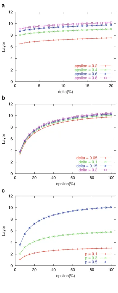
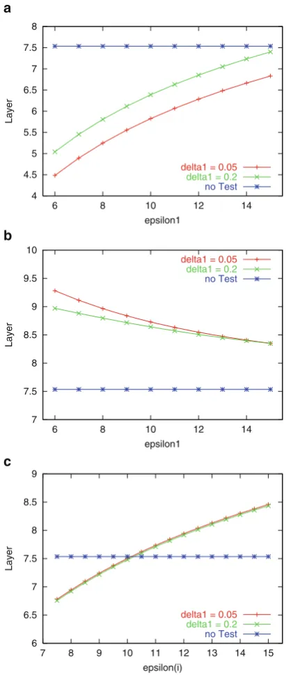
In this chapter, we study the tradeoff between the delay and the accuracy with proving bounds. We implement this study in the context of five key properties of the network, MAX, MIN, QUANTILE, AVERAGE and SUM. Given a user defined accuracy level, we analyze what the layer of the network should be queried for these properties. We show that different queries do show distinct characteristics which affect the delay/accuracy tradeoff. Meanwhile, we present that for certain types of queries such as AVERAGE and SUM, additional statistical information obtained from the history of the environment can help further reduce the number of sensors involved in answering a query. We then investigate the new tradeoffs given the additional information.
The algorithm that we propose for our architecture is fully distributed; there is no need for the sensors to keep information about other sensors. Using the fact that each sensor is independent of others, we show how to balance the power consumption at each node by reconstructing the layered structure periodically, which results in an increase in the life expectancy of the whole network.
3.1.1
Background and Related Work
deployable; its self-organization nature; and its deep penetration to the physical environments. Some surveys on the challenges, techniques and protocols of wireless sensor networks can be found in [1,2,8].
One key objective of wireless sensor network is data collection. Different from data transmission of traditional networking, which is address-based and end-to-end, wireless sensor data collection is data centric, commonly integrated with in-network aggregation. More specifically, each individual sensor contributes its own data and the sensors of the whole network collectively achieve a certain task. There are many research issues related to sensor data collection, in particular, many focus on trade-off between key parameters, such as query accuracy, delay and energy usage (or load balancing).
SPIN [10] is the first data centric protocol which uses flooding; Directed Diffusion [13] is proposed to select more efficient paths. Several related protocols with similar concepts can be found in [5,7,20]. As an alternative to flat routing, hierarchical architectures have been proposed for sensor networks; in LEACH [11], heads are selected for clusters of sensors; they periodically obtain data from their clusters. When a query is received, a head reports its most recent data value. In [24], energy is studied in a more refined way in which a secondary parameter such as node proximity or node degree is included. Clustering techniques are studied in a different fashion in several papers, where [15] focuses on non-homogeneously dispersed nodes and [3] considers spanning tree structures. In-network data aggregation is a widely used technique in sensor networks [18,19,23]. Ordered properties, for example, QUANTILE are studied in [9]. A recent result in [6] considers power-aware routing and aggregation query processing together, building energy-efficient routing trees explicitly for aggregation queries.
Delay issues in sensor networks are mentioned in [16,18] where the aggregation introduces high delay since each intermediate node and the source have to wait for the data values from the leaves of the tree, as confirmed by Yu et al. [25]. In [14], where a modified direct diffusion is proposed, a timer is set up for intermediate nodes to flush data back to the source if the data from their children have not been received within a time threshold. In case of energy-delay tradeoffs, [25] formulates delay-constraint trees. A new protocol is proposed in [4] for delay critical applications, in which energy consumption is of secondary importance. In these algorithms, all of the sensors in the network are queried, resulting in.N/
3.1.2
Chapter Outline
We present the system architecture in Sect.3.2. Section3.3contains the theoretical analysis of the tradeoff between the accuracy of query answers and the latency of the system. In Sect.3.4, we address the energy consumption of our system. Section3.5
evaluates the performance of our system using simulations. We further present some variations of the architecture in Sect.3.6. In Sect.3.7, we summarize this application and how the sublinear algorithms are used in this application.
3.2
System Architecture
3.2.1
Preliminaries
We assume our network has N sensors denoted by s1;s2; : : : ;sN and deployed
uniformly in a square area with side lengthD. We assume that a base station acts as an interface between the sensor network and the users, receiving queries which follow a Poisson distribution with the mean interval length.
We embed a layered structure in our network, with L layers, numbered 0, 1, 2,: : :,L 1. We user.l/to denote the transmission range used on layerl: during a transmission taking place on layerl, all sensors on layerlcommunicate by usingr.l/
and can reach one another, in one or multiple hops. Lete.l/be the energy needed to transmit for layerl. The energy spends per sensor for a transmission ise.l/Dr.l/˛
where2 ˛ 4[22]. Initially, each sensor is at energy levelB, which decreases with each transmission.Rdenotes the maximum transmission range of the sensors.
3.2.2
Network Construction
We would like to impose a layered structure on our sensor network where each sensor will belong to one or more layers. The properties of this structure is as follows.
(a) Thebase layercontains all sensorss1; : : : ;sN.
(b) The layers are numbered 0 throughL 1, with the base layer labelled 0. (c) The sensors on layerlform a subset of those on layerl 1, for1lL 1. (d) The expected number of sensors on each layer drops exponentially with the
layer number.
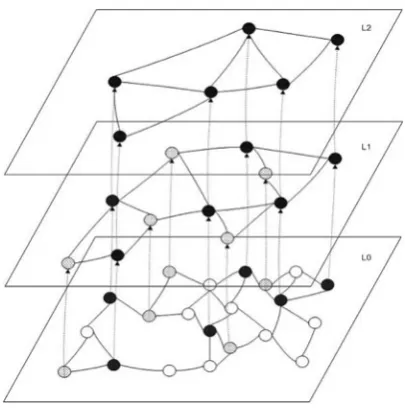
Fig. 3.1 A Layered Sensor Network; a link is presented whenever the sensor nodes in a certain layer are within transmission range
process that a generic sensorsiundergoes. All sensors, includingsi, exist in the base
layer0. Inductively, ifsiexists on some layerl, it will, with probabilityp,promote
itself to layerlC1, which means thatsiwill exist on layerlC1in addition to all
the lower layersl;l 1; ; : : : ; 0. If on some layerl0,si makes the decision not to
promote itself to layerl0C1,sistops the randomized procedure and does not exist
on any higher layers. Ifsi promotes itself to the highest layerL 1, it stops the
promotion procedure since no sensor is allowed to exist beyond layerL 1. Thus, any sensor will exist on layers0; 1; : : : ;kfor some0kL 1. Figure3.1shows the architecture of a sensor network with three layers.
Since our construction does not assume the existence of any mechanism of synchronization, it is possible that some sensors may be late in completing its procedure for promoting itself up the layers. Since the construction scheme works in a distributed fashion, this is not a problem—the late sensor can simply promote itself using probabilitypand join its related layers in its own time.
Whenever the base station has a query, the query is sent to a specific Layer. Those and only those sensors existing on this layer are expected to take place in the communication. This can be achieved by reserving a small field (of log logN
bits) in the transmission packet for the layer number. Once l is specified by the base station (the method for which will be explained later), all of the sensors on layerlcommunicate using transmission ranger.l/. The transmission range can be determined by the expected distance of two neighboring sensors on layer l, i.e.
r.l/ D pD
N=2l, and can be enlarged a little further to ensure higher chances of
3.2.3
Specifying the Structure of the Layers
Note that in the construction of the layers, the sensors do not promote themselves indefinitely; this is because if there are too few sensors on a layer, the inter-sensor distance will exceed the maximum transmission range R. Rather, we “cut off” the top of the layered structure, not allowing more than L layers where
LDlog N
.D
RC1/2
.
In what follows, we assume that the promotion probabilityp D 12. We analyze the effect of varyingpwhen appropriate and in our simulations.
3.2.4
Data Collection and Aggregation
Given a layered sensor network constructed as above, we now focus on how a query is injected into the network and an answer is returned. We simplify the situation by assuming the same as [21] that the base station is a special node where a query will be initiated. Thus the base station acts as an interface between the sensor network and the user.
When the base station has a query to make, it first determines which layer is to be used for this query. Let this layer bel. The base station then broadcasts the query using communication ranger.l/for this layer. In this message, the base station specifies the layer numberl and the query type (in this chapter, we study MAX, MIN, QUANTILE, AVERAGE and SUM). Any sensor on layerl that hears this message will relay information using communication ranger.l/; those sensors not on layerlwill simply ignore this message.
After the query is received by all the sensors on layerl, a routing tree rooted at the base station is formed. Each leaf node then collects its data and sends it to its parent, which then aggregates its own data with the data from its children, relaying it up to its parent. Once the root has the aggregated information, it can obtain the answer to the query.
3.3
Evaluation of the Accuracy and the Number
of Sensors Queried
In this section, we explore how the accuracy of the answers to queries and the latency relate to the layer which is being queried. In general, we would like to be able to obtain the answers to the queries with as little delay as possible. This delay is a function of the number of sensors whose data are being utilized for a particular query. Thus, the delay is reflected by the layer to which the query is sent. We would also like to get as accurate answers to our queries as possible. When a query utilizes data from all the sensors, the answer is accurate; however, when readings from only a subset of the sensors are used, errors are introduced. We now analyze how these concerns of delay and accuracy relate to the number of sensors queried, and thus to the layer used.
To explore the relation between the accuracy of the answer to a query and the layerlto which the query has been sent, we recall that the current configuration of the layers have been reached by each sensor locally, which decides how many layers it will exist. Due to the randomized nature of this process, the number of sensors on each layer is a random variable. In the next lemma, we investigate which layer must be queried if one would like to have input from at leastksensors.
Lemma 3.1. Let l < logN log expected number of sensors on layer l. Then, the probability that there are fewer than k sensors on layer l is less thanı.
Proof. Define random variable Yi for i D 1; : : : ;N as follows.Yi D 1 if si is
promoted to layerl; and Yi D 0 otherwise. Clearly,Y1; : : : ;YN are independent. PrŒYiD 1D 1=2l, andPrŒYiD 0D 1 1=2l. On layerlthere areY D P
N iD1Yi
sensors. Therefore,PrŒY <kDPrŒY < k
EŒYEŒY <e
In what follows, we analyze the accuracy and the layer in the context of certain types of queries.
3.3.1
MAX and MIN Queries
Theorem 3.1. The queries for MAX and MIN must be sent to the base layer to avoid arbitrarily high error.
3.3.2
QUANTILE Queries
As we cannot obtain an exact quantile by querying a proper subset of the sensors in the network we first introduce the notion ofan approximate number of quantile.
Definition 3.1. The-quantile. 2.0; 1/of an ordered sequenceSis the element whose rank inSisjSj.
Definition 3.2. An element of an ordered sequence S is the -approximation -quantileofSif its rank inSis between. /jSjand.C/jSj.
The following lemma shows that a large enough subset ofShas similar quantiles toS.
Lemma 3.2. Let QS be picked at random from the set of subsets of size k of S. Given error boundand confidence parameterı, if k ln2ı
22, with probability at
least1 ı, the-quantile of Q is an-approximation-quantile of S.
Proof. The element with rankjQjinQ1does not have rank within.˙/jSjin Sif and only if one of the following holds: (a) More thanjQjelements inQhave rank less than. /jSjinS, or (b) more than.1 /jQjelements inQhave rank greater than.C/jSjinS.
SincejQj Dk, the distribution of elements inQare identical to the distribution wherekelements are picked uniformly at random without replacement fromS. This is due to the fact that any element ofSis as likely to be included inQas any other element in either scheme, and both schemes includekelements inQ.
Since the two distributions mentioned above are identical, we can think of the construction of Q as k random draws without replacement from a 0–1 box that containsjSj items, of which those with rank less than. /jSjare labelled “1” and the rest are labelled “0”. ForiD1; : : : ;k;letXibe the random variable for the
label of theith element inQ. ThenXDPkiD1Xiis the number of elements inQthat
have rank less than. /jSjinS. Clearly,EŒXD. /k. Hence,PrŒXkD PrŒX EŒXk . /kDPrŒX EŒXkDPrŒXk EŒXk. This is at moste 22k, by Hoeffding’s Inequality. Note that Hoeffding’s Inequality applies to random samples chosen without replacement from a finite population, as shown in Section 6 of Hoeffding’s original paper [12], without the need for independence of the samples.
1Wherever rank in a set is mentioned, it should be understood that this rank is over a sequence obtained by sorting the elements of the set.
Similarly, it can be shown that the probability that more than.1 /jQjelements
We now show which layer we must use for given error and confidence bounds.
Theorem 3.2. If a-quantile query is sent to layer l < logN logln
, then the answer will be the-approximation-quantile of the whole network with probability greater than.1 ı/.
Proof. By Lemma 3.1, the probability that layer l < logN logkCln2ıC
q
ln2ı.2kCln2ı/
has fewer than k sensors is less than ı2. By Lemma 3.2, if
the number of sensor nodes on layer l is at least ln2. 2 ı/
22 D
ln4ı
22, the probabil-ity that the -quantile on layer l is -approximation -quantile of the sensor network is at least 1 ı2. Hence, the answer returned by layer l < logN
log
is-approximation-quantile of the sensor
network with probability greater than.1 ı/. ut
3.3.3
AVERAGE and SUM Queries
3.3.3.1 The Initial Algorithm
AVERAGE queries and SUM queries are correlated queries where the AVERAGE is just SUM=N. Since we know the number of the sensors in advance, we just analyze the AVERAGE queries in this section and do not explicitly explain the SUM queries. We now consider approximating the average data value over the whole sensor network by querying a particular layer. The below lemma indicates that the expectation of the average data value of an arbitrary layer is the same as the average of the base layer, which is the exact average of the sensor network.
Lemma 3.3. Let a1;a2; : : : ;aN be the data values collected by the nodes s1;s2; : : : ;sN of the sensor network. Let k be the number of sensors on layer l. Let X1;X2; : : : ;Xkbe the random variables describing the k data values on layer l. Let XD 1kPkiD1Xi. Then EŒXD N1 PNiD1ai.