www.elsevier.com / locate / econbase
How important is anticipation of divorce in married women’s
labor supply decisions? An intercohort comparison using NLS
data
*
Bisakha Sen
Department of Economics, University of Central Florida, P.O. Box 161400, Orlando, FL 32828, USA Received 4 May 1999; received in revised form 13 September 1999; accepted 23 September 1999
Abstract
I compare two birth-cohorts of married women and find that divorce-risk plays a significantly smaller role in the recent cohort’s labor supply decision. This suggests that any decline in America’s divorce rates will not substantially reduce married women’s labor supply. 2000 Elsevier Science S.A. All rights reserved.
Keywords: Women; Work; Divorce; Intercohort
JEL classification: J16; J22; J12
1. Introduction
It has been argued that one reason behind the growth in married women’s labor supply in the US is the increasing rate of marital instability in American society, and the desire of married women to insure against the economic trauma of divorce by enhancing personal earning capacity. That anticipation of divorce increases married women’s labor supply is well supported in existing literature. Peters (1986) and Parkman (1992) find that residence in unilateral divorce states increases married women’s labor force participation rates. Greene and Quester (1982) and Johnson and Skinner (1986) find that women who perceive themselves as being at greater risk of divorce work more hours in the market.
1
All the above studies use data on women from or prior to the 1970s. Relatively few studies have
*Tel.:11-407-823-2232; fax: 11-407-823-3362.
E-mail address: [email protected] (B. Sen)
1
Peters and Parkman use CPS data on women whose mean age was 44 years in 1979, Greene and Quester use Census Bureau data from 1967, and Johnson and Skinner use PSID data from 1972.
investigated whether labor force behavior of women has changed in more recent times, and to this author’s knowledge, no study has investigated whether the anticipation of divorce continues to play a decisive role in married women’s labor supply decisions in more recent times. Yet, that issue is of interest. Data from recent Statistical Abstracts of the US shows that divorce rates in the country have stabilized since the 1980s, and it is surmised that young people marrying in the 1980s and 1990s will experience lower divorce rates over their lifetimes than their predecessors (Cherlin, 1992). Further-more, there has been a movement towards rolling back unilateral divorce laws in many states (Leland,
2
1996), which could further lower divorce rates in the near future. Hence, if anticipation of divorce is still an important factor in married women’s labor supply decision, then the US could witness a decline in married women’s labor supply before too long.
In this paper, I investigate whether the importance of probability of divorce (divorce-risk) as a factor in women’s labor supply decision has changed across cohorts by comparing the labor supply behavior of married women from the birth cohort 1944–54 to that of married women from the birth cohort 1957–64. I first estimate labor supply equations using the actual incidence of divorce in the near future as an indicator of divorce-risk. Thereafter, to account for the possibility that future divorce is endogenous to current labor supply, I also estimate labor supply equations using two different instruments for divorce-risk (for the theory behind why women’s labor supply may increase divorce-risk, see Becker et al., 1977; Becker, 1981). My results indicate that divorce-risk plays a substantial role in increasing labor supply of married women in the previous cohort, but its impact is significantly smaller for the recent cohort. This suggests that in the previous cohort, ceteris paribus, women who foresaw a high probability of divorce were likely to work more than their low divorce-risk counterparts. However, in the recent cohort, labor supply patterns for high and low divorce-risk women are relatively similar. Therefore, a decrease in divorce rates (and hence perceived divorce-risk) should not cause any momentous decrease in the labor supply of married women in the US.
2. The model
According to Heckman’s (1974) seminal labor supply model, a woman will enter the labor market (that is, her desired hours of work will be positive) if her offered market wage exceeds her zero-hour reservation wage. Accordingly, I define the woman’s desired hours of work (H*) as a linear function of her offered market wage (W ) and zero-hour reservation wage (see Zabel, 1993), where the latterM in turn is defined as a vector of the standard income and demographic variables (Z ) as well as the divorce-risk (P):
H*5lWM1aP1Zb1´ (1)
´ is a well-behaved disturbance term. The well known labor force participation and observed hours equations can thereafter be written, respectively, as:
LFP 51 when lWM1aP1Zb1´.0
(2)
50 otherwise
2
and
Hours 5lWM1aP1Zb1´ when lWM1aP1Zb1´.0
(3)
50 otherwise
The equations can be estimated using probit and maximum likelihood tobit, respectively.
Clearly, higher values of P make not working more risky and hence decrease reservation wages. However, it can logically be argued that the impact of P on labor force participation probabilities is greater in situations where the zero-hour reservation wage is otherwise quite high compared to the market wage, and hence the participation probability is otherwise relatively low. Similarly, if more hours worked in the current period enhance future earning capacity, but do so at a decreasing rate, then the impact of P on hours should be stronger in situations where hours worked in the absence of
3
any divorce-risk are few. Thus, if the reservation wage is lower relative to the offered market wage
for the recent cohort compared to the previous even in the absence of any divorce risk, then the impact of P on participation probabilities and hours should be weaker for the recent cohort compared to the previous. To test whether this is the case, I permit the effect of all variables to vary across cohorts. This is done by including in (2) and (3) the interaction of each variable with a cohort dummy that takes value 0 for the previous cohort and 1 for the recent cohort. The advantage of this method is that it lets the structure of the equations vary fully across cohorts, and permits one to statistically test whether the effect of a particular variable has changed significantly across cohorts. Specifically, the size and significance of the coefficients of (cohort3P) tests the hypothesis of whether the divorce
plays a similar role in the labor force participation and hours decision across cohorts. The equations are first estimated using the actual incidence of divorce within the next three calendar years as a measure of current divorce-risk. Then, to account for the possible endogeneity between divorce and women’s labor supply, the equations are estimated after substituting appropriate instruments (described later in the paper) in place of actual divorce. Since market wages are observed only for women who actually work, predicted market wages estimated via Heckman’s selection-corrected
4
method (1979) are used in the estimations.
3. Data and results
The empirical analysis utilizes sub-samples from the National Longitudinal Survey of Young Women (NLSYW) and National Longitudinal Survey of Youth (NLSY) for the previous and recent cohort, respectively. Since information was only available for years 1979–1993 for the NLSY at the on-set of this study, only the information for 1968–1983 is utilized for the NLSYW to maintain intercohort parity. Furthermore, since the NLSY respondents are aged 14–22 years at time of the first
5
survey, all respondents aged more than 24 in 1968 are dropped from the NLSYW. The selected
3
This is supported by the results of Johnson and Skinner (1986).
4
The wage equation was estimated using schooling, experience, age, race, any health impediment, area of residence, and the selection correction term. Results are available upon request.
5
respondents are civilians who were never married or in their first marriages at the beginning of the survey, and who are observed in the married state, and if divorcing, then in the divorced state, for at least one survey year. Thus, respondents who go either from being single to divorced or from married to divorced to re-married in the space of a single survey are omitted. The event ‘divorce’ is set at 1 if either legal divorce or separation is seen to occur in the space of the next three calendar years, 0 otherwise. Hence, for respondents who do not divorce by 1983 and 1993 for the previous and recent cohort, respectively, the last observations included are from 1980 and 1990.
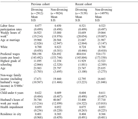
The final sample contains 2937 respondents from the previous cohort of whom 918 get divorced, and 3872 respondents from the recent cohort of whom 1545 get divorced. Pooling all woman-year observations gives 12 736 observations for the previous cohort, of which 2912 observations are contributed by eventual divorcees, and 20 118 observations for the recent cohort, of which 5139 observations are contributed by eventual divorcees. Table 1 gives pooled-observation means of all relevant variables separately for those who eventually divorce and those who do not, by cohort. It can immediately be seen that there is less divergence between hours and participation rates between eventual divorcees and non-divorcees in the recent cohort compared to the previous, and that in fact non-divorcees in the recent cohort register marginally higher hours and participation rates than their eventually divorcing counterparts.
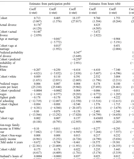
Table 2 presents results from estimating the participation probit and hours tobit models, respectively. The model is estimated on the pooled sample of all women-hour observations from the two cohorts, under the assumption of group-wise heteroskedasticity. The resulting standard errors and
t-statistics are robust to assumptions about the nature of inter-dependence between residual terms for
the same respondent. I first estimate the probit and tobit models using the actual occurrence or non-occurrence of divorce within the next 3 years as a measure of current divorce-risk. I then estimate the equations using the respondent’s age at time of marriage as an instrument for divorce risk. There is strong evidence in the literature that divorce-risk decreases with higher age at time of marriage (see for instance Carter and Glick, 1970; Peters, 1988), probably because marriage at an early age can be associated with an incomplete search process. Hence, it can be inferred that if higher divorce-risk increases labor supply, then a higher age at time of marriage should lower it. Finally, I estimate the equations after substituting predicted probabilities of divorce estimated from an unreported probit model (that uses occurrence of divorce within the next 3 years as dependent variable) in place of
6
actual incidence of divorce in the hours equation.
Results indicate that non-white women are likely to work more than white women, particularly in the previous cohort. Higher wages significantly increases labor supply for both cohorts. However, after accounting for their effect on wages, schooling and age actually decrease hours worked, suggesting that the productivity of non-market time and hence reservation wage is greater for older and better educated women. Of particular interest is the intercohort decline in the negative effects that other family income (including husband’s wage income) and the presence of a young child has on
7
labor supply. The first may indicate a decrease across cohorts in the complementarity between such income and the woman’s non-market time in generating household utility, as well as the growing reluctance among married women to be dependent on their husbands’ incomes. The second may
6
Results are available upon request.
7
Table 1
Means and standard deviations of important variables for divorcing and non-divorcing women using pooled woman-hour
a
Labor force 0.477 0.450 0.521 0.523
participation rates (0.499) (0.498) (0.499) (0.497)
Weekly hours of 16.923 15.080 18.689 19.064
b
work (19.214) (18.976) (20.054) (19.807)
Age at marriage 19.960 20.568 21.047 21.987
(2.826) (2.947) (2.864) (3.147)
White 0.700 0.823 0.724 0.788
(0.458) (0.381) (0.446) (0.410)
Predicted wages 508.198 526.892 484.016 510.173 (cents per hour) (143.492) (153.744) (145.804) (173.530)
Highest grade of 11.895 12.354 11.929 12.523
schooling (2.066) (2.328) (1.881) (2.389)
Age 23.983 25.797 23.747 25.835
(3.703) (3.695) (3.100) (3.275)
Non-wage family
income (including 17.671 19.460 12.795 16.663
husband’s wage (10.567) (11.466) (13.223) (21.048) income) in $‘000s /
year
Child under 6 years 0.622 0.609 0.604 0.611
(0.484) (0.487) (0.498) (0.487)
Husband’s hours of 38.744 40.067 33.400 37.710 work per week (13.216) (12.899) (16.322) (15.018)
Health impediment 0.059 0.052 0.075 0.053
(0.236) (0.220) (0.263) (0.225)
Residence in city 0.401 0.303 0.404 0.366
(0.968) (0.459) (0.491) (0.481)
Residence in the 0.417 0.406 0.447 0.372
south (0.491) (0.491) (0.497) (0.483)
a
Data from the previous cohort is drawn from the NLSYW, and that for the recent cohort is drawn from the NLSY. Means and standard deviations are constructed after pooling observations on all the respondents in the final sample. The means are not adjusted for the over-sampling of disadvantaged whites in the NLSY, which accounts for the lower predicted wages, lower family income, and fewer hours worked by husbands among the recent cohort.
b
Hours worked in survey week, including overtime hours.
reflect access to better child care facilities by the recent cohort compared to the previous, greater participation by husbands in child-rearing, and possibly a change in social attitudes regarding the importance of a mother’s continuous presence in raising a child.
Table 2
Estimates and t-statistics from probit participation equations and tobit hours equations using actual divorce, and age at
a
marriage and predicted divorce probabilities as instruments for divorce
Estimates from participation probit Estimates from hours tobit
Coeff Coeff Coeff Coeff Coeff Coeff
(t-stat) (t-stat) (t-stat) (t-stat) (t-stat) (t-stat)
Cohort 0.713 0.405 18.157 9.760 1.753 29.772
(3.067) (1.576) (27.017) (1.584) (0.264) (26.826)
b
Actual divorce 0.176 4.825
(4.129) (4.505)
b
Cohort3actual 20.148 23.672
divorce (22.859) (22.822)
c
Age at marriage 20.041 20.904
(25.772) (25.191)
c
Cohort3age at 0.015 0.451
marriage (1.952) (2.004)
d
Predicted probability 0.347 11.205
of divorce (3.649) (7.587)
d
Cohort3predicted 20.259 28.622
probability of (22.951) (23.085)
divorce
White 20.207 20.250 20.414 26.410 27.340 27.393
(24.821) (25.852) (22.838) (25.687) (26.596) (4.428)
Cohort3white 0.089 0.110 0.391 2.532 3.084 6.930
(1.651) (2.031) (2.603) (1.796) (2.211) (2.640)
Predicted wages 0.006 0.007 0.004 0.174 0.180 0.068
(cents per hour) (25.210) (25.840) (9.962) (27.693) (28.461) (11.317) Cohort3predicted 20.0004 20.0002 0.004 20.006 20.011 0.108 wages (21.168) (20.577) (9.283) (20.772) (21.285) (13.656)
Highest grade 20.178 20.170 0.288 24.460 24.222 5.521
of schooling (212.719) (212.087) (12.550) (213.518) (212.613) (16.323) Cohort3highest 20.084 20.088 20.540 21.576 21.715 210.753 grade (24.381) (24.560) (220.107) (23.419) (23.679) (223.835)
Age 20.80 20.078 20.158 22.401 22.348 22.460
(213.566) (213.292) (217.020) (214.799) (214.658) (214.530)
Cohort3age 0.002 0.007 0.157 0.43693 0.507 2.144
(0.188) (0.793) (12.955) (1.909) (2.203) (8.536)
Non-wage family
income in $‘000s / 20.10 20.011 20.013 20.277 20.293 20.243 year (27.042) (27.383) (26.945) (27.264) (27.557) (27.793)
Cohort3Non-wage 0.008 0.008 0.013 0.217 0.232 0.257
family income (4.961) (5.252) (6.726) (4.790) (5.036) (7.661)
Child under 6 years 20.672 20.704 20.461 218.575 219.301 29.312 (222.301) (223.009) (211.951) (223.558) (224.355) (214.408)
Cohort3child 0.175 0.178 0.022 5.235 5.443 2.212
(4.417) (4.409) (1.781) (5.174) (5.319) (1.886)
Husband’s hours of 0.0004 20.0001 0.037 0.023 0.012 0.082
work per week (0.325) (20.090) (1.685) (0.821) (0.445) (1.461)
Cohort3husband’s 0.002 0.002 0.003 0.054 0.066 0.519
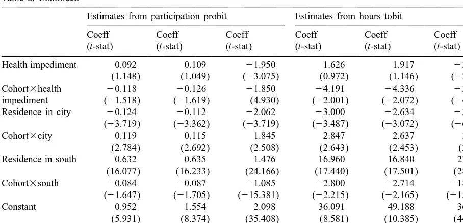
Table 2. Continued
Estimates from participation probit Estimates from hours tobit
Coeff Coeff Coeff Coeff Coeff Coeff
(t-stat) (t-stat) (t-stat) (t-stat) (t-stat) (t-stat)
Health impediment 0.092 0.109 21.950 1.626 1.917 23.471
(1.148) (1.049) (23.075) (0.972) (1.146) (22.249) Cohort3health 20.118 20.126 21.850 24.191 24.336 23.134 impediment (21.518) (21.619) (4.930) (22.001) (22.072) (24.621) Residence in city 20.124 20.112 22.062 23.000 22.634 23.090
(23.719) (23.362) (23.719) (23.487) (23.072) (26.551)
Cohort3city 0.119 0.115 1.845 2.847 2.637 3.535
(2.784) (2.692) (2.508) (2.643) (2.453) (2.404)
Residence in south 0.632 0.635 1.476 16.960 16.840 27.542
(16.077) (16.233) (24.166) (17.440) (17.501) (28.980) Cohort3south 20.084 20.087 21.085 22.800 22.714 218.686
(21.647) (21.705) (215.381) (22.215) (22.165) (215.053)
Constant 0.952 1.554 2.098 36.091 49.188 36.869
(5.931) (8.374) (35.408) (8.581) (10.385) (44.898) Log-likelihood 218733.94 218693.18 215324.75 291363.66 291341.98 287203.85
a
The probit and tobit equations are first estimated using actual incidence of divorce within the next 3 years as the dependent variable. They are then estimated using age at time of marriage and predicted probabilities of divorce as instruments, respectively. The ‘cohort’ dummy takes the value 1 for the recent cohort, 0 for the previous. The dependent variable is hours worked in survey week inclusive of overtime hours. The equations are estimated using GLS under the assumption of group-wise interdependence.
b
Marginal effects calculated at the mean are 0.069 and 20.059, respectively.
c
Marginal effects calculated at the mean are 20.016 and 0.006, respectively.
d
Marginal effects calculated at the mean are 0.137 and 20.101, respectively.
role for the recent cohort. Women in the previous cohort who experience divorce within the next three
8
calendar years have a 7% greater probability of participating in the labor market and work about 4.8 h more per week than those who do not. For the recent cohort, the corresponding numbers are only about 1% and 1.1 h per week. The intercohort differences persist after instruments are substituted for actual divorce. Estimations using age at marriage show that women who marry at higher ages (and are thus at a lower risk of divorce) do indeed work less. For a year’s increase in age at time of marriage, participation probability and hours per week decrease by 1.6% and 0.9 h, respectively, for the previous cohort, but only by 1% and 0.45 h, respectively, for the recent cohort. Finally, a 100% increase in the predicted probability of divorce increases participation probability and hours per week
9
by 13.7% and 11.2 h for the previous cohort, but only by 3.6% and 2.6 h for the recent cohort. The above intercohort differences are all statistically significant.
Thus, it appears that while anticipated divorce-risk was a decisive factor in the labor supply decision of married women in previous times, its impact has declined across cohorts. This suggests
8
Marginal effects are calculated about the variable means. They are presented in the notes below Table 2. The full set of marginal effects is available upon request.
9
that reservation wages of married women before taking into account the divorce-risk have declined over time, so that all married women now work more on average regardless of the possibility of divorce. Possible reasons for this could be greater availability of substitutes for goods produced with a woman’s time, a change in social attitude towards married women (particularly married women with children) working, and greater participation by the husband in household chores. The results suggest that any decline in marital instability in the US in the near future should not, by itself, cause any substantial drop in the labor supply of married women. The results also indicate possible intercohort changes in the effect that married women’s work has on the probability of divorce, which is a subject
worthy of further investigation.
Acknowledgements
This paper is an offshoot of my dissertation. I am grateful to my advisor, Patricia Reagan, to my committee members, GS Maddala, Audrey Light and Dan Levin, and to Randy Olsen, Carolyn Moehling, Bruce Weinberg, Traci Mach, Jeff Yankow and an anonymous referee for many helpful comments and suggestions. I am grateful to the Center for Human Resource Research, Ohio State University, for generously permitting me access to the NLS data and their computing facilities, which greatly facilitated this research. I bear the responsibility for all errors and opinions.
References
Becker, G.S., 1981. In: A Treatise on The Family, Harvard University Press, Cambridge, MA.
Becker, G.S., Landes, E., Michael, R.T., 1977. An economic analysis of marital instability. Journal of Political Economics 85 (6), 1141–1187.
Carter, H., Glick, P.C., 1970. In: Marriage and Divorce: A Social and Economic Study, Harvard University Press, Cambridge, MA.
Cherlin, A.J., 1992. In: Marriage, Divorce, Remarriage, Harvard University Press, Cambridge, MA.
Greene, W.H., Quester, A.O., 1982. Divorce-risk and wives labor supply behavior. Social Science Quarterly 63 (1), 16–27. Heckman, J., 1974. Shadow prices, market wages and labor supply. Econometrica 42 (4), 679–694.
Heckman, J., 1979. Sample selectivity bias as specification error. Econometrica 47 (1), 153–161.
Johnson, W.R., Skinner, J., 1986. Labor supply and marital separation. American Economics Review 76 (3), 455–469. Leland, J., 1996. Tightening the knot. Newsweek, 127 (8), February 19, 1996.
Parkman, A.M., 1992. Unilateral divorce and the labor force participation rate of married women, revisited. American Economic Review 82 (3), 671–678.
Peters, E., 1986. Marriage and divorce: informational constraints and private contracting. American Economic Review 76 (3), 437–454.
Peters, E., 1988. Retrospective versus panel data in analyzing life cycle events. Journal of Human Resources 23 (4), 489–513.