arXiv:1709.06025v1 [physics.soc-ph] 25 Jul 2017
Analysis of High Frequency Impedance
Measurement Techniques for Power Line Network
Sensing
Federico Passerini and Andrea M. Tonello
Abstract—A major aspect in power line distribution networks is the constant monitoring of the network properties. With the advent of the smart grid concept, distributed monitoring has started complementing the information of the central stations. In this context, power line communications modems deployed throughout the network provide a tool to monitor high frequency components of the signals traveling through a power line network. We propose therefore to use them not only as communication devices but also as network sensors. Besides classical voltage measurements, these sensors can be designed to monitor high frequency impedances, which provide useful information about the power line network, as for instance status of the topology, cable degradation and occurrence of faults. In this article, we provide a technical analysis of different voltage and impedance measurement techniques that can be integrated into power line modems. We assess the accuracy of the techniques under analysis in the presence of network noise and we discuss the statistical characteristics of the measurement noise. We finally compare the performances of the examined techniques when applied to the fault detection problem in distribution networks, in order to establish which technique gives more accurate results.
Index Terms—Distribution grids, power line communications modems, impedance measurement methods, reflectometric mea-surement methods.
I. INTRODUCTION
T
HE concept of Smart Grids (SG) refers to the faculty of power grids to operate at the maximum efficiency with the minimum cost in a self-organized fashion, or with minimum human intervention. Within any SG, a huge set of information is sensed and shared throughout the network, then processed by optimization algorithms that subsequently con-trol the network parameters, usually aiming at the maximum efficiency/cost ratio [1]. The first element of this cumbersome chain of operations comprises a network of sensors, whose pre-cision and reliability gives the most fundamental contribution to the overall performance of the SG. The topic of this paper is the study of the accuracy of the measurement performed by the network sensors, and in particular by impedance and voltage sensors.The authors are with the Networked and Embedded Systems Institute, University of Klagenfurt, Klagenfurt, Austria, e-mail: {federico.passerini, andrea.tonello}@aau.at.
A version of this article has been accepted for publication on IEEE Sensors Journal, Special Issue on “Smart Sensors for Smart Grids and Smart Cities”. IEEE Copyright Notice: c 2017 IEEE. Personal use of this material is permitted. Permission from IEEE must be obtained for all other uses, in any current or future media, including reprinting/republishing this material for advertising or promotional purposes, creating new collective works, for resale or redistribution to servers or lists, or reuse of any copyrighted component of this work in other works.
impedance being a more informative quantity than the signal trace measured with the FDR.
Given the growing interest on these measurement tech-niques, the aim of this paper is to shed new light on their applicability and on their accuracy. In particular, given the SG context and the need of smart sensors, we propose to integrate either impedance, FDR orρmeasurements in power line modems (PLM), which are largely deployed in distribution networks to allow power line communications (PLC) [13]. Therefore, PLM will also act also as network sensors.
This paper considers three known impedance measurement methods along with one known method to measure ρor the FDR trace. All these methods are herein revisited with the aim of easy integration within PLM. Consequently, the methods are compared based on typical PLM architectures that operate using different PLC standards, taking into account typical hardware noise sources and giving emphasis to the effects of the medium noise. In fact, the presence of high noise is a major concern in PLC [14] that can act as a severe hurdle to both communication and measurement devices. The effect of the noise is both computed analytically and analyzed via simulations, the prerequisites under which the noise can be considered additive Gaussian are assessed, and the accuracy of these measurements is evaluated in different conditions. More-over, we compare the accuracy of impedance measurements with respect to FDR and reflection coefficient measurements in order to assess which method is the most reliable for network sensing. To this aim, we apply all the presented techniques to the fault detection problem and analyze which technique can detect the fault more accurately.
The rest of the paper is organized as follows. A brief review of the information that can be harvested form single-ended network measurements is presented in Section II. Section III presents the considered impedance measurement techniques and the analytical computation of the effect of noise. The same is done for the FDR andρmeasurements in Section IV. Sec-tion V presents the PLC features that are implemented in the simulation for the comparison of the techniques, whose results are then exposed and commented in Section VI. Conclusions follow in Section VII. As a remark, all the physical quantities and equations that we present in Sections II, III and IV are frequency dependent, but we chose not to explicitly report this dependency to ease the notation.
II. SINGLE-ENDED NETWORK SENSING
In this section, we present the main types of high-frequency measurements that can be performed from a single end and we explain the concepts derived from the transmission line (TL) theory [15] that allow to analyze the measurements for network sensing.
Considering an impedance measurement device plugged to a two-conductor TL, the power line input impedanceZP L is
defined as
ZP L =ZC 1 +ρ
1−ρ =ZC
1 +ρLe−2Γx 1−ρLe−2Γx
(1)
whereZC is the characteristic impedance of the TL,Γ is its
propagation constant,xis the distance from the load.ρis the reflection coefficient defined as
ρ=ZP L−ZC
ZP L+ZC
= VRX
VT X
(2) where VT X is the forward traveling voltage wave, i.e. the
transmitted signal, andVRX is the backward traveling voltage
wave, i.e. the received signal at the same end.ρL is the load
reflection coefficient defined as
ρL=
ZL−ZC
ZL+ZC
(3) whereZL is the load impedance. The load can be either an
appliance/device, a transformer, or simply another TL that bridges the considered TL to the rest of the network. Finally, the so called FDR trace is defined as
T =VRXVT X∗ =ρ|VT X| 2
, (4) which is the Fourier transform of the correlation of the transmitted and received signals in time domain [16]. If we now compare (1), (2) and (4), we see that these formulas can all be derived from each other with a transformation and the application of a scaling factor. It is more important though, to point out that measuring one of these three physical quantities gives the same amount of information about the TL. This is particularly true for the estimation of the line length x. We showed in [17] that taking the inverse Fourier transform (IFT) ofZ measured over a sufficiently wide range of frequencies results in a series of equidistant peaks whose inter-peak distance is a good estimate ofx. When considering a complex network made of a series of branches and interconnections, a similar series of peaks is produced for every branch, resulting at the measurement node in an aggregate series of peaks. Similar works have been published that make use ofρ[10] or
T [8] measurements. These papers show different techniques to preprocess the measured trace in frequency domain and analyze its IFT to estimate the vector x of all the distance between the discontinuities. The knowledge ofx allows then the reconstruction of the network topology using different algorithms. Similar peak analysis based techniques have also been developed to detect and localize the presence of electrical faults in the network [17].
Since ZP L, ρ and T are inter-related, the choice of one
of these quantities for the network sensing resides in the measurement technique to be deployed. In fact, in order to measure ZP L both voltage and current sensing are required,
while measuringρrequires a double voltage sensing. Although measuringρ is equivalent to measuring T when no noise is present, except for a scaling factor, this last measurement has been preferred in the literature because of its simple analog implementation. In fact, T can be measured by multiplying
VT X andVRXwith an analog multiplier and passing the result
through a low pass filter. ρ would require an analog signal divider instead, which is usually far more expensive.
methods range from current and voltage measurements to balancing or resonating networks, including also network analysis. However, not all these methods can be easily imple-mented in a PLC modem for online operation, either because they would require too complex circuitry (balancing bridges) or because they are intrinsically narrow band (resonating networks).
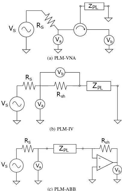
Conversely, easy integration in a PLM front-end can be per-formed for the following techniques: Auto Balancing Bridge (PLM-ABB), current-voltage (PLM-IV), and Vector Network Analyzer (PLM-VNA). We therefore consider a practical implementation where the PLM transmitter is used as the generator of the test signal and the PLM receiver is used as voltmeter. This implies that both the transmitter and the receiver of a given modem are active at the same time.
We are not going to discuss implementation strategies and circuit-related issues of the presented solutions, since these topics have been already tackled in more specialized literature [18], [19]. In this section instead, we explain at system level their operating principles and investigate how the noise affects the measurements. In particular, we concentrate on the effect of the electrical noise coming from the power line channel, since it is the only source of noise that affects the measurement independently of the modem manufacturer. Hence, the results we are going to show have general validity. We also consider the noise due to the digital-to-analog converter (DAC) and line driver at the transmitter, and the noise due to the analog-to-digital converter (ADC) at the receiver, since the resolution of DACs and ADCs might heavily influence the accuracy of the measurements. Other sources of noise, due to the measurement circuit, depend on the specific technology adopted and have to be treated case-by-case.
A. Measurement equations
In the following, the PLM front-end transmitter is modeled with its Thevenin equivalent with ideal source voltageVS and
real source impedanceRS; the power line network is modeled
with its input impedanceZP L, which is in general complex;
two different voltage measures, Va and Vb, are performed
with ideal volt meters. Usually the two voltage measures are performed in series using the same volt meter, to keep the measurement error low. As for this subsection, any kind of noise is neglected.
Let us now consider the PLM-VNA architecture depicted1
in Fig. 1a. The transmitter, the channel and the receiver are connected by means of a circulator or hybrid coupler [20], which also enables full-duplex communication [21]. The main property of the circulator is that it reflects part of the transmitted signal to the receiver scaled by the reflection coefficient
ρ= ZP L−Zo_circ
ZP L+Zo_circ
, (5) whereZo_circ is the output impedance of the circulator at the
channel port. Assuming an ideal circulator, we haveVb=ρVa,
whereVa andVb are the voltages measured at the transmitter
1The depicted circuits are single-ended. Differential implementations are
also possible.
ZPL
Va Vb
VS RS
(a) PLM-VNA
Z
PLVa
Vb
Rsh
VS
RS
(b) PLM-IV
Z
PLVa
Vb Rsh
RS
VS
(c) PLM-ABB
Fig. 1. Basic circuits of the selected impedance measurement methods.
and receiver ports of the circulator, and they corespond toVRX
andVT X of the previous Section respectively.
The main purpose of a VNA is to measure ρ, according to the theory of the scattering parameters [22]. The channel impedance can be also derived from the measured voltages as
ZP L=Zo_circ 1 +ρ
1−ρ =Zo_circ Va+Vb
Va−Vb
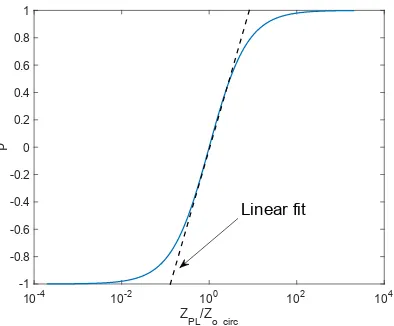
. (6) Modern VNAs can span a very wide range of frequencies, from almost DC to several GHz, using different techniques to implement the hybrid coupler: resistive bridges or active circuits for measurements up to 100 MHz and strip-line couplers for higher frequencies. On the counter side, their sensitivity falls off for impedances whose value is far from
Zo_circ. In fact, when0.1<|ZP L/Zo_circ|<10(see Fig. 2),
ρalmost linearly increases withZP L and so doesVb. Outside
this region the slope ofρ decreases causing minor variations ofVb due to changes in ZP L. This results in a deterioration
of the impedance measurement accuracy.
The PLM-IV and PLM-ABB techniques, depicted in Fig. 1b and 1c respectively, do not suffer the sensitivity problem of the PLM-VNA since they rely on the Ohm’s law, which linearly relates the ratio of the measured voltage and current to the unknown impedance. The PLM-IV technique involves the measurement of the voltageVb at the edges of a shunt resistor,
whose valueRsh is known, in series with the unknownZP L.
This measurement provides the value of the current flowing through ZP L while the voltage across ZP L is given by Va,
ZPL/Zo_circ
10-4 10-2 100 102 104
ρ
-1 -0.8 -0.6 -0.4 -0.2 0 0.2 0.4 0.6 0.8 1
Linear fit
Fig. 2. Relation betweenρandZP Laccording to (5).
In general, Va measured on the transmitter side gives better
results for high values of |ZP L|, while Va measured on the
network side gives better results for low values of|ZP L|[18].
Moreover, in practice Rsh can be replaced with a low loss
transformer that senses the current thanks to the Faraday’s law. Referring to Fig. 1b for the following considerations,ZP Lcan
be derived after simple computations as
ZP L =Rsh
V
a
Vb
−1
. (7) Finally, the PLM-ABB takes its name from the fact that the currentIZP L flowing throughZP L is automatically balanced to the current IRsh flowing through the sensing resistor Rsh by means of an I-V converter. The I-V converter can be a grounded operational amplifier or a more complex integrated circuit. The virtual ground provided by the I-V converter results in a null input impedance. Hence, the current mea-surement is not affected by the network load which gives the PLM-ABB the best high sensitivity range among the three measurement techniques here presented. Referring to Fig. 1c,
ZP L can be derived after simple computations as
ZP L=−Rsh
Va
Vb
. (8)
All the aforementioned techniques can be designed to work in the PLC frequency range (3 kHz – 86 MHz). Since the two voltage measurements needed can be performed by the same volt meter in different time instants, the PLM receiver is enough to absolve this task. Considering the PLM-VNA case, if the modem is used at the same time for full-duplex communication [21] and impedance measurement, the PLM receiver can measure the network impedance only when no analog echo cancellation circuit [23] is integrated in the modem. When analog cancellation is present, it highly corrupts
Vb by renderingρ≃0 in the whole frequency range. Hence,
either the analog echo canceler is fully characterized so that its transfer function can be digitally removed, or a second receiver has to be integrated in the modem to sense the signal before the analog echo canceler.
Va Vb
RS VS
N
VP
N
❩ ✁✂
(a) PLM-VNA
Z
PLVa
Vb
Rsh
RS
VSN VPLN
(b) PLM-IV
Va
Vb
Rsh
RS
VSN
✄PL
VPLN
(c) PLM-ABB
Fig. 3. Noise model of the selected impedance measurement methods.
B. Influence of the noise
In the following, we consider three sources of noise (see Fig. 3):VSN, generated by the transmitter as sum of the DAC, the output filter and the line driver noises;VRN, generated by the ADC at the receiver;VP LN, the equivalent background noise coming from the network [24]. We decided not to include in the following computations the equivalent noise generated by
Rsh, since it only accounts for the noise of one resistor and
is negligible compared to VSN, VRN andVP LN. As already stated, the noise components due to the non-ideality of the circulator and the opamp are not considered.
Considering as before an ideal circulator, the noisy mea-surement using the PLM-VNA provides
Va =Va0+
Ztr_circ
Ztr_circ+RS
VSN+VRN a (9a)
Vb=Vb0+
Ztr_circ
Ztr_circ+RS
ρVSN+
Zo_circ
Zo_circ+ZP L
VP LN+VRN b (9b) where Va0 and Vb0 are the measurements in the absence of
noise as described in Section III-A, and Ztr_circ is the port
(9b) and (6), the measured valueZ¯P L ofZP L becomes whereZP L0 is the ideal network impedance computed using
(6). The above formula shows that the transmitter noise is linearly dependent onZP L and inversely proportional onRS.
The former result is due to the fact that a higher value of
ZP L causes a higher reflection of the transmitted noise to
the receiver; the latter result is due to the voltage partition principle. The amplification of the network noise does not depend on the mismatch between ZP L andZo_circ, but only
onZo_circ. That is because both the measuredVP LN andVb0 are inversely proportional to(Zo_circ+ZP L), but whileVP LN is inversely proportional toVa0,Vb0 is directly proportional to
it. Hence, the effect of (Zo_circ+ZP L)gets canceled.
As for the PLM-IV measurement technique (see Fig. 3b), the measured voltages are
Va =Va0+ When the noise sources are much lower than the signal, (13) can be approximated as
¯
QUALITATIVE DEPENDENCE OFZP LN ON THE CIRCUIT PARAMETERS.
Va0 ZP L RS RshorZo_circ
VNA inverse linear–indep. inverse–indep. indep.–linear RF I-V inverse linear–sigmoid inverse–linear indep.–linear
ABB inverse quadrat.–linear indep.–linear indep.
The above formula shows that the transmitter noise, as for the PLM-VNA case, increases almost linearly with ZP L, while
the network noise has a Sigmoid dependence on its logarithm. Interestingly, the transmitter noise is almost not influenced by
Rsh and it is attenuated, especially for low values of ZP L,
as an inverse function ofRS. On the other side, the channel
noise increases almost linearly withRsh and, for high values
ofZP L, also linearly withRS. From these considerations, it
emerges that, in order to minimize the noise in the PLM-IV impedance measurement technique,Rsh has to be tuned to a
small value, while a balance has to be found forRS in order
to minimize the total noise.
The noisy measurements performed with the PLM-ABB technique (see Fig. 3c) are
Va=Va0+ which, combined with (8), give
¯ When the noise sources are much lower thanVa, (16) can be
approximated as This formula shows that the noise is indipendent ofRsh. This
is due to the decoupling action of the I-V converter. On the other side, the transmitted noise has a quadratic dependence onZP L and the network noise is linearly dependent both on
ZP L andRS.
The dependence of the impedance measurement noise on the circuit parameters are finally summarized in Table I.
C. Modeling of the ADC and DAC noise
As presented in the previous subsections, the measure of
ZP L involves the transformation of a digital test signal to
both the transmitter output noiseVSN and the acquisition noise
VRN for Va and Vb. The influence of these noise sources on the measurements is different based on the measurement approach considered. We differentiate between two different measurement approaches: sequential and cumulated.
In the first approach, pure tones are transmitted sequentially, and a different measurement is performed for every single tone. In this case, the DAC and the ADC can be tuned to exactly clip at the peak amplitude of the transmitted and re-ceived tone respectively. The resulting signal-to-quantization-noise ratio (SQNR) is simply computed from the effective number of bits of the DAC or the ADC. Taking into account also distortion effects of the whole TX and RX chains, PLMs equipped with a 12-bit DAC and a 12-bit ADC, can reach a signal-to-noise-and-distortion ratio (SINAD) of 69 dB at the end of both the TX and RX chains[25].
In the second approach, the test signal is transmitted over all the test frequencies at the same time, and a single broad-band measurement is performed. This is the approach of the orthogonal frequency division multiplexing (OFDM) systems typically deployed in PLC. Although the average generated power may be the same over all the OFDM tones, the peak power of the OFDM signal is much higher than the average power, thus leading to an high peak-to-average-power ratio (PAPR). Hence, the balancing between clipping and quantiza-tion noise highly reduces the SINAD, so that it reaches 60 dB for a 12-bit ADC with an optimum tuning of the parameters [26], [27].
The sequential approach yields the best SINAD but it comes at cost of a much slower acquisition time, whereas the second exploits the features of the PLM to perform a single measurement at a cost of worse SINAD. We remark that in both approaches the transmission time has to be set in order to let the whole network resonate to the transmitted tones. In the following simulations, we focus on the best achievable measurement performance and hence we rely on the sequential approach. The possible use of the cumulated approach is also briefly discussed.
IV. REFLECTION COEFFICIENT ANDFDRMEASUREMENTS
In this section, we briefly analyze a technique to measureρ
andT in order to allow a fair comparison with the impedance measurement techniques presented in Section III.
A direct way to measure ρ and T is to rely on the VNA circuit architecture depicted in Fig. 1a, where the generated signal is forwarded to the network through a hybrid coupler. Different techniques can be applied to properly form the transmitted signal, including the two approaches presented in Section III-C, and to analyze the received one [28]. In our approach, the signalsVa andVbare firstly digitalized and then
(2) and (4) are applied to deriveρandT respectively. When noise is present, as depicted in Fig. 3a, (9a) and (9b) apply. Hence, the resulting noisy reflection coefficient
and trace are
¯
ρ= Vb
Va
≃ρ0+
ρZtr (Ztr+RS)Va0
VSN +VRN b+
+ Zo_circ
(Zo_circ+ZP L)Va0
VP LN =ρ0+ρN (18)
¯
T =VaVb≃ρ|Va0| 2
+ 2ρ Ztr_circ Ztr_circ+RS
Va0VSN+
ρVa0VRN a+
Zo_circ
Zo_circ+ZP L
Va0VP LN+Va0VRN b=T0+TN (19) respectively, taking into account the same approximation used for (11). Here ρ0 andT0 are the quantities of interest, while
ρN andTN are the noise components.
Also in this case the noise is filtered by the presence of the circulator characteristic impedance, the transmitter out-put impedance and the channel impedance. Conversely from impedance measurements, in theT¯ measurement caseVa0 is
now a multiplicative factor for the noise. We remark that, although the error propagation in (18) and (19) is similar, the noise component related toVSN has double amplitude in theT¯ measurement. Moreover,T0is function of the actual reflection
coefficientρ, whileρ0 is only approximately equal to ρ. The
difference is due to the noise caused byVSN andVRN a in the voltage division and is not made explicit in (18), since it is negligible in most of the cases. The effect of these aspects on the overall noise is investigated in detail in Section VI.
V. CONSIDERATIONS ON THEPLCFEATURES In order to assess the performance of the measurement techniques presented in this paper, a closer insight on the PLC characteristics is needed, since PLM operate on frequency ranges and with transmitted power that are specified by PLC standards.
The PL medium has some particular features that differen-tiate it from wired transmission links like telephone twisted-pair cables. First of all, it is made of power cables whose physical characteristics have not been standardized; this means that any cable in a network may have different electrical characteristics that cannot be classified (unlike AWG cables). Secondly, the power cords are not twisted and, more in general, not protected versus possible electro-magnetic interference. Lastly, the loads branched to the PLNs are not matched at PLC frequencies; moreover, they are often time-varying and also produce both thermal and impulsive noise that can be either periodic or not [14]. For theses reasons, the front-end of PLC modems is generally engineered to maximize the voltage sent to the network or received from it [29], instead of maximizing the sent/received power, as in DSL [30]. Hence, the output impedanceRS of both narrowband and broadband
PLC modems has commonly a value ranging from hundreds of mΩs to fewΩs.
SinceRShas a very low value, the transmitted signal has the
or at maximum comparable toZP L. In the case of the
PLM-VNA, it has been shown that to optimize the communication throughput,Zo_circ needs to be matched to the averageZP L
[20].
As already said, ZP L is both frequency and time varying.
While in most of the scenarios it has a periodic time variation that follows the mains cycle, the frequency variation is due to the topological characteristics of the network and can have very complex shapes. In in-home environments, the absolute value of the broadband (2-86 MHz) impedance normally ranges from 50 Ω to 300 Ω [31], while in low-voltage distribution networks the absolute value of the narrowband (3-500 kHz) impedance can go down to few Ω[32].
Finally, VP LN is a major issue in PLCs because of its im-pulsive nature and possibly high value. However, the imim-pulsive noise component ofVP LN might not necessarily compromise the accuracy of the measurement. In fact, impedance mea-surements can be performed during the time windows where impulsive noise is not present and its transients are also ended. Otherwise, their effect can be mitigated by averaging many measurements over time. As for the background noise, it can be described as a complex colored Gaussian process (CCGN), with power spectrum inversely proportional to the frequency. Different measurement campaigns have been performed to measure the noise both in MV distribution lines [33], LV distribution lines [34] and in-home environments [35]. They show that the background noise spans on average from -60 dBm/Hz to -110 dBm/Hz in the narrowband, and from -110 dBm/Hz to -140 dBm/Hz in the broadband. This information is useful when compared to the transmitted power allowed by the communications standards.
The IEEE standard for narrowband PLC limits the max-imum voltage injected into the network in the Cenelec fre-quencies (3 to 148.5 kHz) in the range 97 dBµV/Hz to 110 dBµV/Hz, based on the frequency sub-band [36]. The same standard also limits the maximum power that can be transmitted in the FCC band (150 kHz to 500 kHz) in the range -45 dBm/Hz to -55 dBm/Hz, depending on the frequency. In reference to broadband PLC, the IEEE standard [37] limits the maximum power that can be transmitted to -55 dBm/Hz in the 2 MHz 30 MHz band and to 85 dBm/Hz in the 30 MHz -86 MHz band. All the aforementioned values are referred to a standard load impedance whose value is RSL =50 Ω for
the FCC bands and the broadband PLC, andZSL=50Ω\\ (5 Ω+ 50µH) for the Cenelec bands [38], where \\ denotes the parallel operator on two impedances.
VI. COMPARISON OF THE MEASUREMENT TECHNIQUES Considering all the relations presented in Sections III and IV, we can now compare the three impedance measurement techniques, the ρ measurement and the FDR techniques in terms of overall error. In particular, we define the quantity (of interest)-to-noise ratio (QNR) as
QN R= E h
|X0|
2i
Eh|XN|
2i, (20)
whereE[·] is the expectation operator andX can be either
ZP L, ρ, or T. This relation is more useful than the simple
noise variance, since it normalizes the noise variance with the magnitude of the true data, thus providing an easily comparable result.
In order to set a fair comparison, we consider the transmit-ters of the three circuits under analysis to produce the same voltage and power on the test loadRSL. This causes the three
methods to generate differentVS, since the output impedance
towards the network is different. In particular, using the same value ofRS, the ABB method generates the lowestVS. It is
then the one that generates the lowestVSN and consumes less power.
To have a uniform voltage and power reference for the whole PLC bands, we use RSL as a common impedance
reference. Since the Cenelec bands use the reference loadZSL
instead (see Section V), their maximum allowed voltage has to be converted. The limit voltageVmax_Rfor the Cenelec bands
referred toRSL is
Vmax_R=
RSL
RSL+RScmp
ZSL+RScmp
ZSL
Vmax_Z, (21)
where Vmax_Z is the limit voltage for the Cenelec bands
referred to ZSL and RScmp is the overall output impedance
of the modem seen from the network. With this conver-sion,Vmax_R ranges from 97 dBµV/Hz to 114 dBµV/Hz, or
equivalently the maximum transmitted power ranges from -10 dBm/Hz to 7 dBm/Hz.
As for the network noise, we generate it as shown in the Appendix. The power spectral density needed for the noise generation can be obtained from the power profiles presented in Section V as follows. The noise power profiles are generally referred to the input impedance of a spectrum analyzer, which is RSA=50Ω. If we call PSA the noise power measured by
the spectrum analyzer and PP LN the average power of the network noise, then
PP LN =
(RSA+ZP L)
RSA
PSA. (22)
As forVSN andVRN, we assume the modem to be equipped with a 10-bit DAC and a 12-bit ADC, so that the noise at the output of the transmitter is 55 dB belowVS [39] and the noise
at the end of the receiver chain is 69 dB below Va and Vb
respectively.
In the following, (10), (13), (16), (18) and (19) will be thoroughly analyzed in different conditions.
A. Comparison in terms of transmitted power
In this subsection, we consider fixed impedance values and show how the QNR varies as function of the channel noise powerPP LN and of the powerPT X onZP L. In particular, we setZP L =Ztr_circ =50Ω,Zo_circ=100Ω,Rsh=RS =
1 Ω.
PPL
and low transmitted power though, the QNR of the PLM-ABB and PLM-IV methods declines more rapidly.
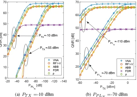
Considering now the ADC and DAC noise components (see Section V), the situation changes. The plots of Fig. 5 show the QNR trends for PT X and PP LN values that are typical of narrowband (PT X =-10 dBm, PP LN =-70 dBm) and broadband (PT X =-55 dBm, PP LN =-110 dBm) PLC. All the techniques tend to saturate to the QNR for which the contribution of VSN becomes greater than that of VP LN. The FDR curves saturate far below the others. This is due to the fact that, according to (19), T0 is the exact value of
the FDR trace, while ρ0 and ZP L0 measured with all the
considered techniques are actually perturbed by a small error caused mostly by VSN which is not rendered explicit in the simplified equations (11), (14), (17) and (18). This error is negligible for low QNRs, but at higher QNRs tends to balance the noise contribution due toVSN inρN andZP LN. SinceT0 is an exact value, the same balancing does not apply toTN.
We finally point out that, using the cumulated measurement approach instead of the sequential one, the ADC noise is
ℜ❬ ✟
increased, thus fixing the saturation of the QNR to lower values.
B. Comparison in terms of impedance value
In this subsection, we consider fixed PT X and PP LN values and show how the QNR varies as function of ZP L.
In particular, we set PT X = -10 dBm, PP LN = -70 dBm,
Rsh=RS =1Ω,Ztr_circ=50 Ω,Zo_circ=100Ω.
According to the results of the previous subsection, for high impedance values the PLM-VNA method has the highest QNR. However, Fig. 6 shows that its accuracy decreases for lower impedance values. This is due to the fact that when
ZP L ≪ Zo_circ the numerator in (6) becomes very small,
thus enhancing the effect of the noise. Conversely, the QNR of the PLM-ABB and PLM-IV methods is maximum for low values and slowly decreases for higher values. Below 10Ωthe PLM-ABB method has the best QNR, while the QNR of the PLM-IV method shows a decreasing trend. This is due to the fact that for this comparison we considered the configuration that is more suited for high impedance measurements. Fig. 6 also shows that the QNR value in only slighted affected by the immaginary part ofZP L for all the methods considered.
As for the FDR andρmeasurement techniques, we notice that whenZP L=Zo_circthe QNR in dB goes to−∞. This is due
to the fact that in this caseVb0 = 0: since a multiplication or a
division is performed to derive T andρrespectively, this will result in a pure noise component.
C. Additive Gaussian noise limits
ZPL [Ω]
7 shows the maximum power of the PL noise for which
¯
ZP LN is additive Gaussian. The maximumPP LN is steeply proportional to PT X and increases almost exponentially with
ZP L. However, the limits shown are higher than the normal
power line background noise values. For example, if PT X =
-10 dBm and ZP L =100, Z¯P LN measured with the PLM-ABB technique is perturbed by additive Gaussian noise when
PP LN <-40 dBm, which is on average true. We conclude that average impedance measurements performed on power grids should provide results perturbed with additive Gaussian noise. The null value of the FDR method is again due to the fact thatT is the result of a multiplication (19), yielding overall a mixed sum of Gaussian and Chi-square distributions. When
PP LN is low, the DAC noise dominates in the Chi-square pairs, which therefore degenerate to Gaussian variables. The opposite is valid when PP LN is high. Hence, although the FDR technique provides the worst accuracy in terms of QNR, it provides the best Gaussian profile, i.e. it is the simplest to analyze and simplify.
D. Application to fault detection
In this subsection, we show the results obtained by applying all the aforementioned measurement techniques to the problem of detecting a fault in a Smart Grid. This way, we assess the performance of each technique in a concrete application.
As presented in [17], an electric fault can be detected in power grids by continuously sensing the impedance over a wide spectrum. More in general, a fault can be detected by continuously sensing the network by means of any reflecto-metric method and then analyzing the function
∆ = 100·
pdenote the fault and pre-fault conditions. If∆is greater than a certain threshold defined by the user at a certain frequency, then its inverse Fourier transform (IFT) δ(t) can give useful information about the fault properties. In particular, the first
freq [Hz] ×105
(a) Impedance based method
freq [Hz] ×105
(b)ρbased method
Fig. 8. ∆generated by either a high impedance or a very far fault.
time [s] ×10-5
(a) Impedance based method
time [s] ×10-5
(b)ρbased method
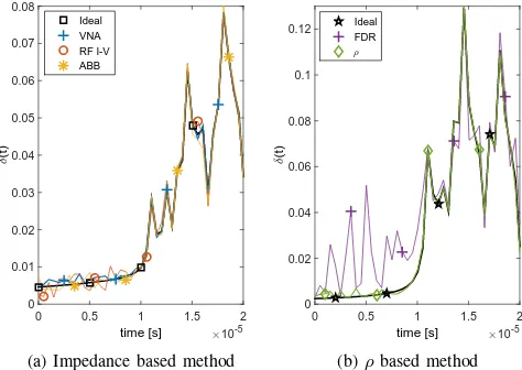
Fig. 9. δ(t)generated by either a high impedance or a very far fault.
peak ofδ(t)indicates the return time of the echo caused by the fault. If the propagation velocity inside the network is known, then the return time can be converted in the distance of the fault.
In order to test the different measurement techniques pre-sented in this paper, we simulated the presence of a fault whose occurrence results in low values of∆. Such a fault can be either characterized by a very high impedance or simply occur far away from the measurement point. The test signal and the power line noise are set at -55 dBm and -120 dBm respectively. Looking first at the ideal measurements in Fig. 8, we note that the values of ∆ given by an impedance measurement are in general lower compared to those given by a measurement ofρ. This is due to the fact that, while ρ
can linearly track changes of impedance along the network,
ZP L undergoes lower variation when very low or very high
the performance of the FDR method is significantly worse. This is due to the different level of noise saturation reached by every method (see Fig. 5). The analysis of δ(t) reveals some further insight: while the impedance measured with the PLM-VNA method almost perfectly coresponds to the ideal trace, the PLM-IV and PLM-ABB methods are characterised by a higher level of noise in the first part and eventually fail to identify a secondary peak. The noise of theρmeasurement in the first part is comparable to that of the PLM-ABB method, while the noise of the FDR method is so high that a correct identification of the first peak is impossible.
As expected from the preliminary analysis of the previous subsections, the impedance measured with the PLM-VNA method also gives the best results when applied to the fault detection problem. The PLM-ABB, PLM-IV, and ρmethods provide similar results in terms of noise, but the ρ measure-ment provides higher values of ∆ resulting in easier fault detection. Finally, the FDR method provides almost only noise data for such low values of ∆.
VII. CONCLUSIONS
In this paper, we proposed to integrate an additive circuit in the front-end of power line communications modems, which allows them to act as high frequency network sensors. We took under analysis three different circuit architectures: the PLM-VNA, the PLM-ABB and the PLM-IV. They enable to measure three quantities: impedance, reflection coefficient and FDR trace. In order to assess the accuracy of such measurements, we analyzed the effect of both the power line channel noise and the PLM noise. The results showed that for low channel impedance values the best accuracy in terms of QNR is obtained by the impedance measured with the PLM-ABB architecture, while the one measured with the PLM-VNA architecture is the best elsewhere. In this context, we showed the values of QNR that are expected for common levels of transmitted signal power and noise in both narrowband and broadband PLC. In particular, we found the limits for which the QNR is dominated by the power line noise and by the PLM noise respectively. We also showed that, when applied to PL in the presence of background noise, all the presented techniques provide measurements perturbed by additive Gaussian noise.
Finally, we applied the different measurement techniques to the problem of fault detection. This application confirms the best performance of the impedance measured with the PLM-VNA architecture, and also points out that the widely used FDR technique gives the worse results among the other considered techniques. In conclusion, the choice of the archi-tecture to be integrated in a PLM and the type of measurement to be performed is based on the kind of network that has to be sensed. For low voltage distribution grids, where the impedance has often very low values, we suggest to perform network sensing by measuring the network impedance with either the PLM-ABB or the PLM-IV architectures; for medium voltage distribution grids or indoor grids, where the impedance ranges from tents to hundreds Ω, we suggest to measure the network impedance with the PLM-VNA architecture.
APPENDIX
Since in this paper all the formulas are frequency dependent and we want to compare different measurement methods at each frequency, the noise has to be defined in frequency domain. From the stochastic processes theory, the Fourier transformX(f)of a stationary processx(t)with autocorrela-tionR(t1, t2) =R(τ)whereτ =t1−t2, and power spectrum
S(ω), is a random process with the following properties [41]: 1) The meanm(f)ofX(f)is the Fourier transform of the
mean m(t) =m0 ofx(t), namely
m(f) =m0δ(f) (23)
2) The autocorrelationΓ(f1, f2)ofX(f)is
Γ(f1, f2) = 2πS(f1)δ(f1−f2) (24)
hence the Fourier transform of a stationary process is a non-stationary white process with spectral density 2πS(f1).
Moreover, since we are considering Gaussian noise processes, their Fourier transform are still Gaussian processes. Therefore, using also (24), the noise at each frequencyfiis uncorrelated
to the other frequencies, and it is a complex Gaussian variable with variance σ2
N = 2πS(fi). Since the average power
spectrum is known from different measurement campaigns (see Section V), the complex Gaussian noise can be generated for each frequency using for example the Box-Muller method [42].
When the noise is generated in frequency domain, any colored power spectral density can be accurately reproduced, and the relative noise in time domain can be simply obtained by performing the inverse Fourier transform of the generated noise. If we now consider, as it happens in real systems, that the signal is transmitted at discrete frequencies, the noise process generated with this method becomes continuous periodic in time domain. In order to avoid time aliasing and the consequent power spectral density alteration, the frequency step has to be short enough to letR(τ)reach negligible values before the following periodic repetition.
REFERENCES
[1] S. F. Bush, Smart grid – communication-enabled intelligence for the electric power grid. Wiley, 2014.
[2] X. Fang, S. Misra, G. Xue, and D. Yang, “Smart grid – the new and improved power grid: A survey,” IEEE Communications Surveys Tutorials, vol. 14, no. 4, pp. 944–980, Fourth 2012.
[3] S. Das, S. Santoso, A. Gaikwad, and M. Patel, “Impedance-based fault location in transmission networks: theory and application,”IEEE Access, vol. 2, pp. 537–557, 2014.
[4] M. Sedighizadeh, A. Rezazadeh, and I. Elkalashy, “Approaches in high impedance fault detection – a chronological review,”Advances in Electrical and Computer Engineering, vol. 10, no. 3, pp. 114–128, 2010. [5] M. N. Alam, R. H. Bhuiyan, R. A. Dougal, and M. Ali, “Design and application of surface wave sensors for nonintrusive power line fault detection,”IEEE Sensors Journal, vol. 13, no. 1, pp. 339–347, Jan 2013. [6] A. Primadianto and C. N. Lu, “A review on distribution system state estimation,”IEEE Transactions on Power Systems, vol. PP, no. 99, pp. 1–1, 2016.
[8] M. Ahmed and L. Lampe, “Parametric and nonparametric methods for power line network topology inference,” inPower Line Communications and Its Applications (ISPLC), 2012 16th IEEE International Symposium on, March 2012, pp. 274–279.
[9] K. Zhang, “Performance assessment for process monitoring and fault detection methods,” Ph.D. dissertation, Duisburg-Essen University, 2016. [10] C. Neus, “Reflectometric analysis of transmission line networks,” Ph.D.
dissertation, Vrije Universiteit Brussel, 2011.
[11] F. Passerini and A. M. Tonello, “Power line fault detection and localiza-tion using high frequency impedance measurement,” in2017 Interna-tional Symposium on Power Line Communications and its Applications (ISPLC), April 2017.
[12] ——, “On the exploitation of admittance measurements for wired network topology derivation,” IEEE Transactions on Instrumentation and Measurement, vol. 66, no. 3, pp. 374–382, March 2017.
[13] S. Galli, A. Scaglione, and Z. Wang, “For the grid and through the grid: The role of power line communications in the smart grid,”Proceedings of the IEEE, vol. 99, no. 6, pp. 998–1027, June 2011.
[14] L. Di Bert, P. Caldera, D. Schwingshackl, and A. M. Tonello, “On noise modeling for power line communications,” in2011 IEEE International Symposium on Power Line Communications and Its Applications, April 2011, pp. 283–288.
[15] C. Paul, Analysis of Multiconductor Transmission Lines, ser. Wiley - IEEE. Wiley, 2008. [Online]. Available: https://books.google.at/books?id=uO5HiV6V8bkC
[16] B. C. de la Torre, “Dsl line tester using wideband frequency domain reflectometry,” Master’s thesis, University of Saskatchewan, Saskatoon, Canada, 2004.
[17] F. Passerini and A. M. Tonello, “Power line fault detection and localization using high frequency impedance measurement,” in 2017 IEEE International Symposium on Power Line Communications and its Applications (ISPLC), April 2017.
[18] L. Callegaro,Electrical Impedance: Principles, Measurement, and Ap-plications. CRC Press, 2012, ISBN: 9781439849101.
[19] “Agilent impedance measurement handbook – 4th ed.” 2013. [Online]. Available: "http://cp.literature.agilent.com/litweb/pdf/5950-3000.pdf" [20] F. Passerini and A. M. Tonello, “In band full duplex PLC: The role of
the hybrid coupler,” in2016 International Symposium on Power Line Communications and its Applications (ISPLC), March 2016, pp. 52–57. [21] G. Prasad, L. Lampe, and S. Shekhar, “In-band full duplex broadband power line communications,” IEEE Transactions on Communications, vol. 64, no. 9, pp. 3915–3931, Sept 2016.
[22] D. M. Pozar,Microwave Engineering – Fourth Edition. John Wiley & Sons, 2011.
[23] T.-C. Lee and B. Razavi, “A 125-mhz mixed-signal echo canceller for gigabit ethernet on copper wire,”IEEE Journal of Solid-State Circuits, vol. 36, no. 3, pp. 366–373, Mar 2001.
[24] M. Antoniali, A. M. Tonello, and F. Versolatto, “A study on the optimal receiver impedance for SNR maximization in broadband PLC,”Journal of Electrical and Computer Engineering, vol. 2013, 2013.
[25] Analog Devices, Broadband Modem Mixed-Signal Front End. AD9866 datasheet, 2016. [Online]. Available:
http://www.analog.com/media/en/technical-documentation/data-sheets/AD9866.pdf
[26] H. Ehm, S. Winter, and R. Weigel, “Analytic quantization modeling of ofdm signals using normal gaussian distribution,” in2006 Asia-Pacific Microwave Conference, Dec 2006, pp. 847–850.
[27] C. R. Berger, Y. Benlachtar, R. I. Killey, and P. A. Milder, “Theoretical and experimental evaluation of clipping and quantization noise for optical ofdm,” Opt. Express, vol. 19, no. 18, pp. 17 713–17 728, Aug 2011. [Online]. Available: http://www.opticsexpress.org/abstract.cfm?URI=oe-19-18-17713 [28] T. W. Monteith, “Locating telephony loop impairments with frequency
domain refectometry,” Master’s thesis, University of Saskatchewan, Saskatoon, Canada, 2002.
[29] M. De Piante and A. M. Tonello, “On impedance matching in a power-line-communication system,”IEEE Transactions on Circuits and Systems II: Express Briefs, vol. 63, no. 7, pp. 653–657, July 2016. [30] P. Golden, H. Dedieu, and K. Jacobsen,Implementation and Applications
of DSL Technology. CRC Press, 2007, ISBN: 9780849334238. [31] M. Antoniali and A. M. Tonello, “Measurement and characterization
of load impedances in home power line grids,”IEEE Transactions on Instrumentation and Measurement, vol. 63, no. 3, pp. 548–556, March 2014.
[32] I. H. Cavdar and E. Karadeniz, “Measurements of impedance and attenuation at cenelec bands for power line communications systems,”
Sensors, vol. 8, no. 12, pp. 8027–8036, 2008. [Online]. Available: http://www.mdpi.com/1424-8220/8/12/8027
[33] Z. Tao, Y. Xiaoxian, Z. Baohui, N. H. Xu, F. Xiaoqun, and L. Changxin, “Statistical analysis and modeling of noise on 10-kv medium-voltage power lines,”IEEE Transactions on Power Delivery, vol. 22, no. 3, pp. 1433–1439, July 2007.
[34] Y. Xiaoxian, Z. Tao, and Z. Baohui, “Measurement and research of the characteristics of noise distribution in three-phase four-wire low-voltage power network channels,”IEEE Transactions on Power Delivery, vol. 22, no. 1, pp. 122–128, Jan 2007.
[35] R. Hashmat, P. Pagani, A. Zeddam, and T. Chonavel, “Mimo com-munications for inhome plc networks: Measurements and results up to 100 mhz,” in2010 IEEE International Symposium on Power Line Communications and Its Applications, March 2010, pp. 120–124. [36] “IEEE standard for low-frequency (less than 500 khz) narrowband power
line communications for smart grid applications,” 2013.
[37] “IEEE standard for broadband over power line networks: Medium access control and physical layer specifications,” 2010.
[38] “Signalling on low-voltage electrical installations in the frequency range 3 khz to 148,5 khz – part 1: General requirements, frequency bands and electromagnetic disturbances,” 2012.
[39] ST Microelectronics, Power-line communication, analog front-end. ST-PLC-AFE datasheet, 2016. [Online]. Available: www.st.com/resource/en/datasheet/DM00252996.pdf
[40] W. Daniel,Applied nonparametric statistics, 2nd ed. Cengage Learning, 2000.
[41] A. Papoulis and S. U. Pillai, Probability, Random Variables, and Stochastic Processes, 4th ed. McGraw-Hill Higher Education, 2002. [42] G. E. P. Box and M. E. Muller, “A note on the generation of random