DELINEATION OF SUB-PIXEL LEVEL SEDIMENTARY LITHO-CONTACTS
BY SUPER RESOLUTION MAPPING OF LANDSAT TM IMAGE
Shanmuga Priyaa S*, Sanjeevi S
Remote Sensing Unit, Department of Geology, Anna University, Chennai, INDIA [email protected]
KEY WORDS: Super resolution mapping, Litho-contact delineation, Linear spectral unmixing, Spectral angle mapper, Hopfield neural network
ABSTRACT:
To delineate the geological formation at the surface, satellite image classification approaches are often preferred. This study aims to produce a super resolved map with better delineation of the litho-contacts from the medium resolution Landsat image. Conventionally used per-pixel classification provides an output map at the same resolution of the satellite image, while the super resolved map provides the high resolution output map using the medium resolution image. In this study, four test sites are considered for delineating different litho-contacts using super resolution mapping approach in Cuddalore district, southern India. The test sites consists of charnockite, fissile hornblende-biotite gneiss, marine sandstone and sandstone with clay, limestone with calcareous shale and clay, clay with limestone bands/lenses, mio-pliocene and quaternary argillaceous and calcareous sandstone, fluvial and fluvio-marine formations. This work compares the per-pixel, super resolved output derived from linear spectral unmixing (LSU) based HNN and spectral angle mapper (SAM) based HNN approaches. The super resolution mapping approach was performed on the medium resolution (30m) Landsat image to obtain the litho-contact maps and the results are compared with the existing maps and observations from field visits. The results showed improved accuracy (90.92%) of the map prepared by the SAM based super resolution approach compared to the LSU based super resolution approach (90.14%) and the maximum likelihood classification approach (83.74%). Such an improved accuracy of the super resolved map (6m resolution) is due to the fact that the lithological mapping is done not merely at the resolution of the image, but at the sub-pixel level. Hence, it is inferred that super resolution mapping applied to multispectral images may be preferred for mapping lithounits and litho-contacts than the conventional per-pixel and sub-pixel image classification methods.
1. INTRODUCTION
Visual interpretation of multispectral and hyperspectral satellite images has long known to be a potential technique for lithological and litho-contact mapping. Many instances of updation of the existing geologic maps by satellite image interpretation have been reported from around the world (Krishnamurthy, 1997; Hadigheh and Ranjbar, 2013). Classification approaches are often preferred to delineate the geological formation at the surface using satellite images. Though this is an accepted approach, the coarse spatial resolution of many satellite images leads to inaccurate portrayal of the litho-contacts. This issue was addressed in the late 80s and spectral unmixing/sub-pixel classification was suggested as a classification approach to overcome such limitations (Sanjeevi, 2008). Later, it was realized that spectral unmxing techniques can only result in resolving the sub-pixel issue but cannot resolve the location of the classes within a pixel. This lacuna resulted in the evolution of the super resolution approach which not only identifies the number of classes within a coarse resolution pixel, but also exactly specifies the location of classes within a pixel (Atkinson, 2005).
This paper reports a study which aims to produce a super resolved map with better delineation of the litho-contacts from the medium resolution Landsat image. The conventionally used per-pixel classification provides an output map at the same resolution of the satellite image, while the super resolved map provides the higher resolution output map using the medium resolution image. In this study, four test sites in Cuddalore
district, southern India are considered for delineating the different litho-contacts by the super resolution mapping approach.
Super resolution mapping (SRM) is achieved by integrating linear spectral unmixing (LSU) and spectral angle mapper (SAM) with the Hopfield Neural Network (HNN) approach. The end-member pixels representing the lithological units were identified by the pixel purity index method. These end-member pixels were used to generate the fraction images and the distance measure images by the LSU and SAM technique respectively. These fraction images and the inverse distance measure images are given as inputs to the HNN based super resolution mapping. The 30m resolution Landsat TM image resulted in a super resolved output of 6m resolution that clearly delineates most of the litho units and litho-contacts in the study area.
This work also compares the per-pixel output and super resolved output derived from the LSU-based SRM technique and the SAM-based SRM technique. The quality of the outputs (lithologic maps) from the LSU and SAM based super resolution mapping approaches, performed on the medium resolution (30m) Landsat images, is evaluated by comparing with the existing geological maps and from observations made during the field visits.
2. PREVIOUS STUDIES
Lithological mapping has been attempted using remote sensing techniques such as FCC, PCA, colour transformation etc. The International Archives of the Photogrammetry, Remote Sensing and Spatial Information Sciences, Volume XL-8, 2014
(Krishnamurthy, 1997). It is presently done using supervised per-pixel classification (Bishta et al, 2013) and band ratio techniques (Madani and Emam, 2011). Mineral abundance mapping applications are now being attempted by sub-pixel classification such as linear spectral unmixing (Sanjeevi, 2008). Landsat Thematic Mapper (TM) imagery has been used for mineral mapping and exploration because the two shortwave infrared (SWIR) bands are useful for predicting alteration mineral associations (Sabine, 1997).
Hadigheh and Ranjbar (2013) compared MLC, SAM and SID for lithological mapping from ASTER and IRS data in the Eastern part of the central Iranian volcanic belt. The authors preferred MLC (Maximum Likelihood Classification) than SAM (Spectral Angle Mapper) and SID (Spectral Information Divergence) classification approaches in their study.
Zhang and Pazner (2007) applied maximum likelihood classification for ASTER, Hyperion and Landsat ETM data in the Southeastern Chocolate Mountains, USA. To get an accurate lithology maps, Zhang and Pazner, (2007) suggested that it requires high resolution spatial and spectral information and extensive field surveys.
3. STUDY AREA
Four test sites in Cuddalore district, southern India are considered for delineating the different litho-contacts by the super resolution mapping approach. The study sites consist of charnockite, fissile hornblende-biotite gneiss, marine sandstone and sandstone with clay, limestone with calcareous shale and clay, clay with limestone bands/lenses, mio-pliocene and quaternary argillaceous and calcareous sandstone, fluvial and fluvio-marine formations. The Cuddalore sandstone of mio-pliocene age is surrounded by cretaceous formations of clay and limestone, recent fluvial and fluvio-marine formations (Figure 2).The robustness of the classification approach is evaluated by choosing study sites in such a way that there exists more than one lithotype in each site.
4. DATA USED
The multispectral Landsat 5 TM (Thematic Mapper) for classification approaches such as per-pixel, sub-pixel and super resolution mapping. Landsat TM image has the spatial resolution of 30m and 7 number of bands (Table 1). Landsat images are atmospherically corrected and georeferenced images.
Bands 6 of Landsat image is not considered in this study due to its incompatible spatial resolution (b6=120m).
Parameters Landsat 5 TM
Spectral Range 0.45-2.35
Spatial Resolution 30m
Swath Width 185Km
Spectral Resolution 190-250nm
Spatial Coverage Non-continuous
Total number of bands 7
Date of Acquisition of image 25th August 1991 Table 1. Sensor specification of Landsat
Figure 2. Geological map of the study area (GSI, 1995) 5. METHODOLOGY
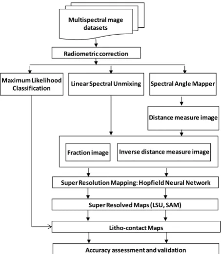
In this work, super resolution mapping is achieved by integrating linear spectral unmixing (LSU) and spectral angle mapper (SAM) with the Hopfield Neural Network (HNN) approach (Figure 3). The end-member pixels representing the lithological units were identified by the scatterplot method (Schowengerdt, 1997). These end-member pixels were used to generate the fraction images and distance measure images by the LSU and SAM technique respectively. These fraction images and the inverse distance measure images are given as inputs to the HNN based super resolution mapping.
Figure 1. Location of study area depicting the four sites in the Cuddalore region, southern India Veeranam Eri
Perumal
R. Kollidam ARABIAN
SEA
.
DelhiChennai.
.Cuddalore
BAY OF BENGAL
2 1
3
4
Study site 3- Fluvial without vegetation and Sandstone with clay
Study site 4- Fluvial and Fissile hornblende-biotite gneiss
Study site 2- Fluvial with vegetation, paleochannel and Sandstone with clay Study site 1- Argillaceous and calcareous sandstone, Clay with limestone bands/lenses and Sandstone with clay
Cuddalore
.
.Neyveli
Super Resolution Mapping: Hopfield Neural Network
Super Resolved Maps (LSU, SAM)
Litho-contact Maps
Linear Spectral Unmixing Spectral Angle Mapper
Fraction image
Distance measure image Multispectral mage
datasets
Inverse distance measure image Radiometric correction
Accuracy assessment and validation Maximum Likelihood
Classification
Figure 3. Flowchart depicting the methodology of the study 6. PER-PIXEL CLASSIFICATION
Per-pixel classification assumes that each pixel represents a single land cover class or lithotype only. It ignores the mixed pixel problem. In per-pixel classification (or hard classification) algorithms, each pixel is individually grouped into a certain category. Per-pixel classifiers develop a signature by combining the spectra of all training set pixels for a given feature. Per-pixel or hard classification can give high accuracy only if the scene is homogeneous or the image used is of high spatial resolution so that a single pixel consists of a single class.
Maximum likelihood classification assumes that the statistics for each class in each band are normally distributed and calculates the probability that a given pixel belongs to a specific class. Each pixel is assigned to the class that has the highest probability (Jenson, 1986).The maximum likelihood classifier (MLC) has long been used by many authors in the field of geological mapping (Rowan and Mars, 2003), agriculture (Heller & Johnson 1979, Keene & Conley 1980), landcover mapping (Yuan and Elvidge 1998), urban mapping (Ridd 1995, Jensen and Cowen 1999), water body/ wetland mapping (Ramsey and Laine 1997, Lunetta and Barlogh 1999). Most of the authors have mentioned that the maximum likelihood approach was adopted because of its robustness, versatility, higher accuracy.
7. SUB-PIXEL CLASSIFICATION INPUTS 7.1 Linear Spectral Unmixing
Spectral mixing occurs either during image acquisition or resampling. In higher resolution images, the percentage of mixed pixels may reduce but they still occur in the boundary pixels. Linear spectral unmixing is used to infer the proportions of the pure components that gave rise to the mixed pixel. The mixed pixels can be spectrally unmixed through various techniques such as linear spectral unmixing (Settle & Drake 1993; Sanjeevi 2008); fuzzy c means classification (Foody
1996) and fuzzy supervised classification (Zhang & Foody 2001).
The steps involved in linear spectral unmixing are: 1. Selection of appropriate End members 2. Unmix the image by Linear Spectral Unmixing. 3. Generation of fraction Images.
Equation (1) represents the linear mixing model for a pixel in an image with i number of bands.
(1) where:
Ri is a composite reflectance of the mixed spectrum in band i; Fj is a fraction of end-member (j) in the mixture;
Rf is a reflectance of that end-member in band i; n is number of end-members;
e is an error in the sensor band i;
Based on the above equations, Linear Spectral Unmixing technique is applied to the Landsat TM image and the fractions of rock types in each pixel is computed.
4.1.1 Fraction images: The abundance of classes in each pixel can be shown in the form of fraction images. The end-member pixels are chosen from the scatter plot of PC1 vs PC2 (Schowengerdt 1997). The appropriate end-member spectra for each class must be chosen in such a way that the fraction image depicts the exact abundance of the class within the pixel. The brighter pixel in the fraction image indicates the presence of larger proportion of the class in the pixel and the darker pixel indicates the presence of small or no proportion of class in that pixel. These fraction images are the input for LSU based SRM. 7.2 Spectral Angle Mapper
SAM is a spectral classifier that utilizes an n-D angle to match pixels to the reference spectra (Kruse et al 1993). The algorithm determines the spectral similarity between two spectra by calculating the angle between the spectra and treating them as vectors in a space with dimensionality equal to the number of bands. SAM compares the angle between the end-member spectrum vector and each pixel vector in the n-D space. The spectral set of a satellite image is given as X={x1, x2…, xn} ⊂ Rq, the reference spectral set r= {r1, r2.., rc} ⊂ R
q
, both x and r are the non-zero vector, where q is the number of spectral bands, n is the number of pixels, c is reference spectrum of the classes in the image. The spectral angle or spectral similarity measure (Beatriz et al, 2008), θcxn= {θki} (k=1,…,c, and
i=1,…,n) between the pixel spectra xi and the reference
spectrum rk is defined as:
θki= cos -1
(xi·rk)/(||xi || ·||rk||) (2) Smaller angles represent closer matches to the reference spectrum. SAM algorithm uses only the vector direction and not the vector length (Liu and Yang, 2013). The result of the SAM classification is an image showing the best match at each pixel. Many authors used SAM for geological mapping (Rowan and Mars, 2003; Van Der Meer et al, 2010; Hadigheh and Ranjbar, 2013).
7.2.1 Inverse distance measure images: The spectral angle mapper provides a distance measure image, where a smaller distance indicates a closer match with the reference spectra, and a larger distance indicates no or lesser match with the reference spectra. This distance measure image indicating the closeness to the reference spectra is the inverse in appearance of the abundance image. Here the darker pixel indicates the high abundance and brighter pixel represents the low abundance of the land cover class in that pixel.
For obtaining the area proportion or abundance image, the distance measure is inverted (Equation 3). This inverted distance measure image of SAM is used as an input for the HNN based SRM.
Inverse distance image=1-float (Distance measure image) (3) 8. SUPER RESOLUTION MAPPING
In this work, super-resolution mapping is achieved by integrating the linear spectral unmixing and spectral angle mapper with the Hopfield Neural Network approach. Hopfield Neural Network is a feed-forward and fully connected recurrent neural network wherein each neuron is modeled using an input and a sigmoidal activation function. The Hopfield network can be used for energy minimization problems if the weights and biases are arranged such that they describe an energy function, with the minimum of energy occurring at the stable state of the network (Tatem et al, 2002).
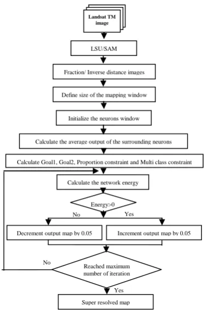
Mapping the spatial distribution of class components within each pixel is formulated as a constraint satisfaction problem with an optimal solution determined by the minimum of the energy function. From the Landsat image at 30m spatial resolution, a set of proportion images for each rock type is obtained by the linear spectral unmixing. The flowchart for the super-resolution mapping approach is given in Figure 4. Each pixel in the image input into the neural network is to be processed by a set of 5 X 5 (25) neurons. The network for each pixel processing is constructed with 25 neurons, since a zoom factor of 5 is adopted.
The neurons are given an initial value as follows:
If a pixel has an area proportion for a particular landcover class as 100%, all neurons are given a value of 0.55. Similarly, if a pixel has an area proportion for particular landcover class as 50%, 13 neurons are given a value of 0.55 and 12 neurons are given a value of 0.45. The concept of spatial order within and outside a pixel is the basis for determining the energy of the network. The point at which minimum energy occurs is the stable state of the network. The neuron outputs at this point determine the best accurate map of the given image. The network energy function based on the goal and constraints of the sub-pixel level mapping task given in Equation (4) as:
E = - ∑ ∑ (k1G1 + k2G2 +k3P+k4M (4)
where k1, k2, k3 are constants weighting the various energy parameters taken a value of 1; G1 and G2 are output values for neuron of the two objectives (or) goal functions; P is the output value for neuron of the proportion constraint; M is the output value of the neuron for multi-class constraint,
, where is the average
output of jth class for sub-pixel at position (i,j). The first goal function is given in Equation (5) as:
G1(i,j)=floor(1+tanh(average(surrounding 8 neurons output)-0.5))) * (neuronoutput(i,j) – 1.0 (5) This goal function aims to increase the output of the central neuron to 1 if the average output of the surrounding eight neurons was greater than 0.5. If the averaged output of the neighboring neurons is less than 0.5, the goal function evaluates to 0, and has no effect on the energy function. If the averaged output is greater than 0.5, the goal function evaluates to 1 and the neuron output controls the magnitude of the negative gradient output, with only neuron output of 1 producing a zero gradient. A negative gradient is required to increase the neuron output, when the output = 0 and the mean of surrounding 8 neurons is greater than 0.5.
Figure 4. Flowchart depicting the methodology for Super resolution mapping of multispectral satellite images The second goal function is given in Equation (6) as:
G2(i,j) = (1-floor(1+tanh(average(surrounding 8 neurons output)-0.5))) * neuronoutput(i,j) (6) This goal function aims to decrease the output of the central neuron to 0, given that the average output of the surrounding eight neurons was less than 0.5.The tanh function evaluates to 0 if the averaged output of the neighboring neurons is more than 0.5. If it is less than 0.5, the function evaluates to 1 and the central neuron output controls the magnitude of the positive gradient output. If the neuron output = 0, the second goal function produces a zero gradient.
P=floor((1+tanh (neuronoutput(i,j)-0.5)))-p(i,j) (7) where, p(i,j) is the estimated proportion
A positive gradient is required to decrease the neuron output when the neuron output is 1 and the average of the surrounding eight neurons is less than 0.5.
When neuron output=1 and average of surrounding 8 neurons is greater than 0.5, G1=0.
When neuron output=0 and average of surrounding 8 neurons is less than 0.5, G2=0.
Energy = G1 + G2 = 0
This energy function satisfies the objective of the super-resolution mapping task, while also forcing the neuron output to either 0 or 1 to produce a bipolar map of the given image. The proportion constraint is used to check whether the area proportion estimate of each pixel of the input image is maintained during the energy minimization process (super-resolution mapping task). A positive P value (Equation 7) is
No
LSU/SAM
Yes No
Yes
Landsat TM image
Fraction/ Inverse distance images
Define size of the mapping window
Initialize the neurons window
Calculate the average output of the surrounding neurons
Calculate Goal1, Goal2, Proportion constraint and Multi class constraint
Reached maximum number of iteration
Super resolved map
Decrement output map by 0.05 Increment output map by 0.05 Energy>0
Calculate the network energy
produced if proportion estimate exceeds the actual value and a negative P value is produced if proportion estimate is less than the actual value. When the proportion estimate is equal to the actual initial value, P=0 and E=0. The super resolved fraction or proportion image is obtained for each class. This proportion image produces the super-resolved classified map. The above steps and equations are scripted in MATLAB® environment.
9. RESULTS AND DISCUSSIONS 9.1 Results of MLC
It has been emphasized many times that per-pixel classification assumes that each pixel represents a single land cover class only and it ignores the mixed pixel problem. Per-pixel or hard 2003; Hadigheh and Ranjbar, 2013) but acceptable results have not been obtained. MLC results for the four test sites show the crisp output at 30m resolution where it is unable to delineate the exact boundary between the lithotypes.
9.2 Results of LSU based SRM
The results of LSU as the input for super-resolution mapping of LANDSAT image for four sites are shown in Figure 5 and 6. It can be seen from the fraction images that regions fully occupied by a litho-type are represented by bright pixels, while in the mixed pixels, those that have another litho-type are represented by dark or black pixels. The boundary pixels or mixed pixels that fail to delineate the litho-contacts in per-pixel classification, exhibit varying shades of grey, indicating the presence of other litho-types in these pixels.
Though the abundance of the lithotypes in the boundary is correctly quantified, the vegetation cover in some areas is misclassified as a lithotype. The results show that the accuracy of SRM from LSU depends on the end- members and the number of classes present within the scene. The LSU works well when the PC scatter plot provided three end-member pixels with distinct spectral separability. The only limitation of the LSU is choosing appropriate end-members.
9.3 Results of SAM based SRM
The same training pixels were given as input for all the soft classification approaches. The proportion of litho-classes present in each pixel is given as the inverse distance image (Figure 5 and 6). The closeness of two or more classes results in similar inverse distance images for those classes. In the inverse distance image for a lithotype, brighter pixels indicate that they are spectrally closest to that class pixel given as input and the distance measure is inversely proportional to the abundance of class in the pixel.
9.4 Accuracy assessment and validation
Since this study involves evaluation of super-resolution mapping as a potential tool to accurately map the litho-contacts, it is pertinent that the classification has to be accurately performed. Hence, the first step could be to evaluate the accuracy of the classification (by comparing with existing lithology maps of the study sites), and the next step would be to
check the validity of the results. The results of the accuracy
assessment indicating the producer’s, user’s and overall
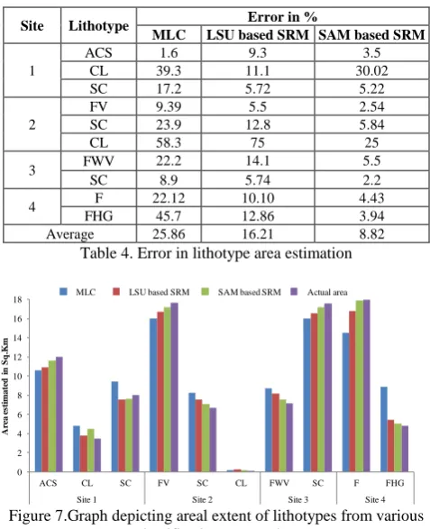
accuracy, and kappa statistics for the three outputs from LANDSAT image for four different sites are provided in Table 2. The results are validated by estimating the area for each lithotypes in the study sites (Table 3). Table 4 represents the error in estimation of areal extent of lithotypes from MLC, LSU based SRM and SAM based SRM approaches. It is also depicted in the form of graph as shown in Figure 7. The overall error indicates that SAM based SRM approach outperforms the LSU based SRM and the conventional MLC approaches.
Site Litho
UA-User’s Accuracy; PA-Producer’s Accuracy; OA-Overall Accuracy;
KS-Kappa Statistics; ACS-Argillaceous and Calcareous Sandstone; CL-Clay with Limestone; S-Sandstone; FV-Fluvial with vegetation; SC- Sandstone with clay; FWV-Fluvial without vegetation sediments; F-Fluvial sediments; FHG-Fissile Hornblende Gneiss
Table 2. Accuracy Assessment for per-pixel, LSU based SRM and SAM based SRM outputs
Table 3. Comparison of areal extent of lithotypes mapped by various classification approaches
10.CONCLUSIONS
This study has demonstrated that the super resolution mapping approach outperforms the per-pixel classification approach in the context of litho-contact identification and mapping in a sedimentary terrain. An important factor that aided in accurate mapping and delineation of the lithounits and their contacts is the presence of the SWIR band in Landsat TM image data. The carbonate rich cretaceous formation exhibits SWIR absorption, while the iron rich lateritic mio-pliocene sandstone exhibits absorption in the NIR region.
Landsat TM FCC image
Per-pixel output Fraction images LSU based SRM Inverse distance images SAM based SRM Actual lithology map
(GSI, 1995)
Figure 5. Per-pixel, LSU based SRM and SAM based SRM results for the sites1 and 2 in Cuddalore region, southern India
Site 1
Clay with limestone bands Sandstone with clay
Argillaceous and calcareous sandstone
Clay with limestone bands Sandstone with clay
Argillaceous and calcareous sandstone
Site 2
Sandstone with clay
Clay with limestone bands Alluvium with vegetation
Sandstone with clay
Clay with limestone bands Alluvium with vegetation
The
Inter
national
Archiv
es
of
the
Photog
rammetr
y,
Remote
Sensing
and
Spatial
Inf
or
mation
Sciences
,
V
ol
ume
XL-8,
2014
ISPRS
T
echnical
Commission
VIII
Symposium,
09
–
12
December
2014,
Hyder
abad,
India
T
h
is
co
n
tri
b
u
tio
n
h
a
s
b
e
e
n
p
e
e
r-re
vi
e
w
e
d
.
d
o
i:1
0
.5
1
9
4
/isp
rsa
rch
ive
s-XL
-8
-1
3
8
9
-2
0
1
4
1
3
9
Landsat TM FCC image
Per-pixel output Fraction images LSU based SRM Inverse distance images SAM based SRM Actual lithology map
(GSI, 1995)
Figure 6. Per-pixel, LSU based SRM and SAM based SRM results for the sites 3 and 4 in Cuddalore region, southern India
Site 3
Site 4
Fluvial Fissile hornblende-biotite gneiss Fluvial Fissile hornblende-biotite gneiss
Legend
Argillaceous and calcareous sandstone
Clay with limestone bands/ lenses Fissile hornblende-biotite gneiss Quaternary Fluvial sediments
Quaternary Fluvio-Marine sediments Limestone with calcareous shale and clay Quaternary Marine sediments
Sandstone Sandstone with clay
Fluvial without vegetation Sandstone with clay Fluvial without vegetation Sandstone with clay
The
Inter
national
Archiv
es
of
the
Photog
rammetr
y,
Remote
Sensing
and
Spatial
Inf
or
mation
Sciences
,
V
ol
ume
XL-8,
2014
ISPRS
T
echnical
Commission
VIII
Symposium,
09
–
12
December
2014,
Hyder
abad,
India
T
h
is
co
n
tri
b
u
tio
n
h
a
s
b
e
e
n
p
e
e
r-re
vi
e
w
e
d
.
d
o
i:1
0
.5
1
9
4
/isp
rsa
rch
ive
s-XL
-8
-1
3
8
9
-2
0
1
4
1
3
9
Site Lithotype Error in %
Table 4. Error in lithotype area estimation
Figure 7.Graph depicting areal extent of lithotypes from various classification approaches
The lithocontacts mapped by the SRM approach match well with the actual lithocontacts seen in the maps published by GSI (1995). The average error in the areal extent of the lithotypes computed by SAM based SRM is 8.82% compared to 16.21% and 25.86% of LSU based SRM and per-pixel respectively. Apart from accurate delineation of the lithocontacts, the accuracy of image classification is also better for the SRM (SAM-90.92%, LSU- 90.14%) approach than the MLC (83.74%) approach. Such an improved accuracy of the super resolved map (6m resolution) is due to the fact that the lithological mapping and litho-contact mapping is done not merely at the pixel level of the image, but at the sub-pixel level. Hence, it is inferred that super resolution mapping applied to multispectral images may be preferred for mapping lithounits and litho-contacts than the conventional per-pixel and sub-pixel image classification methods.
REFERENCES
Atkinson, P. M., 2005. Super-resolution target mapping from soft classified remotely sensed imagery. Photogrammetric Engineering and Remote Sensing, 71(7), pp.839-846.
Beatriz ,G. P., Conde, O. M., Jesús, M., Cubillas, A. M., & López-Higuera, J.M. 2008. Data processing method applying principal component analysis and spectral angle mapper for imaging spectroscopic sensors. IEEE Sensors Journal, 8, pp. 1310–1316.
Bishta, AZ., Sonbul, AR., & Kashghari, W. 2013. Utilization of supervised classification in structural and lithological mapping of Wadi Al-Marwah Area, NWArabian Shield, Saudi Arabia. Arabian J of Geosciences, doi:10.1007/s12517-013-1044-9 Foody, G.M., 1996. Approaches for the production and evaluation of fuzzy land cover classifications from remotely sensed data. International Journal of Remote Sensing, 17(7), pp. 1317-1340.
GSI (Geological Survey of India), 1995. Geological and Mineral map of Tamilnadu and Pondicherry. Kolkatta: Geological survey of India publication.
Hadigheh, S.M.H. & Ranjbar H. 2013. Lithological mapping in the Eastern part of the central Iranian volcanic belt using combined ASTER and IRS data. Journal of Indian Society of Remote Sensing, 41(4), pp.921-931.
Krishnamurthy, J. 1997. The evaluation of digitally enhanced Indian Remote Sensing Satellite (IRS) data for lithological and structural mapping, International Journal of Remote Sensing, 18(16), pp. 3409-3437.
Kruse, F. A., Lefkoff, A. B., Boardman, J. B., Heidebrecht, K. B., Shapiro, A.T., Barloon, P.J., & Goetz, A.F.H., 1993. The Spectral Image Processing System (SIPS) - Interactive Visualization and Analysis of Imaging spectrometer Data. Remote Sensing of the Environment, 44, pp. 145-163.
Liu, X. & Yang, C., 2013. A Kernel Spectral Angle Mapper Algorithm for Remote Sensing Image classification. 6th International congress on image and signal processing (CISP 2013), pp. 814-818.
Madani, A. A. and Emam, A. A, 2011. SWIR ASTER band ratios for lithological mappingand mineral exploration: a case study from El Hudi area, southeastern desert, Egypt. Arabian journal of Geosciences, 4, pp.5-52.
Rowan, L.C. and Mars, J.C., 2003, Lithologic mapping in the Mountain Pass, California area using Advanced Spaceborne Thermal Emission and Reflection Radiometer (ASTER) data. Remote Sensing of Environment, 84, pp. 350–366.
Settle, JJ., & Drake N.A., 1993. Linear mixing and the estimation of ground cover proportions. International Journal of Remote Sensing, 14, pp. 1159–1177.
Sabine, C. 1997. Remote sensing strategies for mineral exploration. A.E. Rencz (Ed.), Remote Sensing for Earth Sciences, John Wiley & Sons, Inc., New York, pp. 375–447 Sanjeevi, S., 2008.Targeting Limestone and Bauxite Deposits in Southern India by Spectral Unmixing Of Hyperspectral Image Data, The International Archives of the Photogrammetry, Remote Sensing and Spatial Information Sciences, 37(B8). Schowengerdt, RA., 1997. Remote Sensing models and methods for image processing. Elsevier (USA).
Tatem, AJ, Lewis, HG, Atkinson, PM & Nixon, MS 2002. Super resolution land cover pattern prediction using a Hopfield
neural network’, Remote Sensing Environment, 79 (1), pp.1-14.
Van Der Meer, F., Vazquez-Torres, M. and Van Dijk, P. M. 1997. Spectral characterization of ophiolite lithologies in the Troodos Ophiolite complex of Cyprusand its potential in prospecting for massive sulphide deposits, International Journal of Remote Sensing, 18(6), pp.1245-1257.
Zhang, J., and Foody, G. M. 2001. Fully-fuzzy supervised classification of sub-urban land cover from remotely sensed imagery: statistical neural network approaches. International Journal of Remote Sensing, 22, pp. 615–628.
Zhang X, Pazner, M 2007. Comparison of Lithologic Mapping with ASTER, Hyperion, and ETM Data in the Southeastern Chocolate Mountains, USA. Photogrammetric engineering and remote sensing, 73(5), 555-561.
MLC LSU based SRM SAM based SRM Actual area