EVALUATION OF DEM GENERATION ACCURACY FROM UAS IMAGERY
M. Santise*, M. Fornari, G. Forlani, R. Roncella
DICATeA, Università di Parma, Viale delle Scienze 181/a, 43124 Parma, Italy
(marina.santise, matteo.fornari2)@studenti.unipr.it, (gianfranco.forlani, riccardo.roncella)@unipr.it
Commission V, ICWG I/Vb
KEY WORDS: UAS, Photogrammetry, Cartography, Accuracy, DEM/DTM, Comparison
ABSTRACT:
The growing use of UAS platform for aerial photogrammetry comes with a new family of Computer Vision highly automated processing software expressly built to manage the peculiar characteristics of these blocks of images. It is of interest to photogrammetrist and professionals, therefore, to find out whether the image orientation and DSM generation methods implemented in such software are reliable and the DSMs and orthophotos are accurate. On a more general basis, it is interesting to figure out whether it is still worth applying the standard rules of aerial photogrammetry to the case of drones, achieving the same inner strength and the same accuracies as well. With such goals in mind, a test area has been set up at the University Campus in Parma. A large number of ground points has been measured on natural as well as signalized points, to provide a comprehensive test field, to check the accuracy performance of different UAS systems. In the test area, points both at ground-level and features on the buildings roofs were measured, in order to obtain a distributed support also altimetrically. Control points were set on different types of surfaces (buildings, asphalt, target, fields of grass and bumps); break lines, were also employed. The paper presents the results of a comparison between two different surveys for DEM (Digital Elevation Model) generation, performed at 70 m and 140 m flying height, using a Falcon 8 UAS.
* Corresponding author. This is useful to know for communication with the appropriate person in cases with more than one author.
1. INTRODUCTION
However spectacular its success, research and development in Unmanned Aerial Systems (UAS) or drones is still ongoing. Originally born from the army sector, the technology of these vehicles is continuously improving and showing its usefulness in countless civil applications, from film making to agriculture (Berni et al., 2009; Gini et al., 2012), from power lines maintenance (Pagnano et al, 2013) to surveillance. Currently, two main factors limit the scale of its application: the operating range provided by battery power and, ironically, the spectacular success of these vehicles, that is finally prompting the airspace regulators to step in and provide necessary guidelines both on the mandatory technical features required on-board and on the UAS operation modes.
Being aerial photogrammetry the main technique used in the production of technical maps, thanks to the high productivity and uniform precision of restitution, there is an obvious interest for the photogrammetric use of UAS; also in Digital Elevation Models (DEM) production, though laser scanning has an obvious edge on forested areas, photogrammetry is regaining ground, thanks to improvements in automatic image orientation and to new techniques for DEM generation that deliver dense and detailed products with resolutions that match or even overcome those of laser scanning.
It is probably too early to define the limits for the use of UAS in these two fields; the main constraints will likely come from the regulations from the airspace authority in terms of operating volume (maximum ground distance from the control station and maximum relative height). This will affect the practicability and the economics of the surveys with UAS, especially in urban areas, where it might find a chance in large scale map updating if the restrictions are not too strict. In other survey applications,
such as quarry and open pits monitoring, where safety issues are not as demanding (González-Aguilera et al., 2012), it might successfully compete with terrestrial laser scanning.
The growing use of UAS platform for aerial photogrammetry comes with a new family, highly automated, processing software capable to deal with the characteristics of these blocks of images. It is of interest to photogrammetrist and professionals, therefore, to find out whether the image orientation algorithms and the Digital Surface Model (DSM) generation methods implemented in such software are reliable and the DSMs and orthophotos are accurate.
2. TEST AREA & UAS PLATFORM
2.1 Area of study
Being a rather new technology at least for civil applications (Eisenbeiss, 2009), few specifications are available concerning technical prescriptions and operation guidelines for UAS surveys. Right now, just a few works were presented concerning the costs of UAS cartographic surveys based on their extension, in order to find the tipping point from conventional airborne photogrammetry and UAS photogrammetry. As the area of interest increase in size so does the time necessary to complete the survey, due to the short operating time range of the majority of these devices (except, perhaps, the fuel-powered ones that are however less and less used in these applications) and to the low flying speed achievable by rotor based ones; more spare batteries and on-site recharging becomes necessary; this makes the ground operations more and more expensive. At the same time, in many countries, national UAS flight regulations limit the area that can be covered with a single operation: for
example, in Italy, the National Commercial Aviation Authority (Ente Nazionale per l’Aviazione Civile – ENAC) imposes that the pilot maintains a strictly visual line of sight of the UAS flight, and the flying area is smaller than 500x500 m2. Moreover, with wider image blocks, considering the large number of images and that currently the navigation solution of all the available commercial UAS is not enough accurate to provide direct orientation parameters, the ground control survey should provide an appropriate number of GCPs (Ground Control Point) to ensure a good image block rigidity.
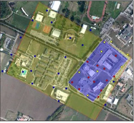
Figure 1: The area used for the case studies. In light yellow the 140 m high flight zone, in blue the 70 m flight zone. Yellow,
blue and red dots show the GCPs used respectively for both case studies, only for the 140 m flight and only for the 70 m
flight.
For all these reasons, the survey for the case studies was restricted to an area of about 500x500 m2; this size might well represent a case where a cartographic update procedure performed with the use of UAS systems can efficiently substitute a traditional photogrammetric flight. The area of study covers part of the Campus of Parma University, for a total of about 2300 m2 and consists of parking lots, green areas, sporting facilities as well as buildings of various heights (from 6 to 35 m). From this point of view, the area can exemplify both an urban and/or a countryside or suburbs scenario. In this paper two different case studies are presented: the first, implementing a 140 m height flight (Italian regulations limit to 150 m the maximum flight altitude for UAS commercial systems) with a Ground Sampling Distance (GSD) of 4 cm/pixel, spanning the whole area; the second, with a 70 m altitude (2 cm/pixel GSD), limited to a 500 m2 region where the most buildings are located (see Figure 1).
2.2 The UAS and the camera used
The employed drone is a Falcon 8 optacopter, produced by the German company AscTec (see Table 1 for specifications). The drone has a fairly good flying autonomy being able, with common payload, to fly up to 20 minutes in automatic way. Nonetheless, for the larger of the two areas, four subsequent flights were required to cover the entire area while also the smaller had to be divided in 2 subzones as well also due to the peculiar execution of the flight plan implemented in the
navigation software. Rather than shooting with the platform in motion, the navigation software of the Falcon drives the UAS to each waypoint, where it stops while shooting the image.
Falcon 8 technical specifications
Weight 0.75 kg
Payload capacity 2.2 kg Flight duration 20 min Flight radius max. 500 m Flight altitude max. 150 m
Table 1 – Technical specifications of UAS Falcon 8.
The Falcon flew with a pre-planned flight whose strips run parallel to the shorter side of the areas. In order to avoid holes and guarantee an overabundant stereoscopic coverage, the longitudinal overlap was fixed to 80% and the side one to 40%. As will be further explained in the next sections, one of the most critical aspect involving this kind of survey is that not always the estimated overlap is observed (even with a carefully designed flight plan), especially in urban environments where abrupt height changes have to be expected. Given the on-board camera characteristics and mounting (see below), the camera station waypoints were planned according to a base length ca. 13 m for the 70 m flight and ca. 25 m for the 140 m flight. A total of 104 images were obtained for the smaller area, divided in 8 strips (4 strips for each subzone), and 128 for the larger area in 16 strips (see Table 2 and Table 3).
Table 2 – UAS flight plan characteristics at 140 m.
Table 3 – UAS flight plan characteristics at 70 m.
The camera installed on the UAS is a compact Sony NEX-5 (Sensor APS CMOS Exmor™) with a resolution of 14.2 Mpixel, image frame 21.6 x 14.4 mm, pixel size 4.7 micrometers and a fixed focal length of 16.3 mm. To reduce the payload, the camera is powered by the battery pack of UAS. This complicated a little the calibration of the optics, since also
Flight at 140 m
the image acquisition for the calibration must be performed with the camera connected to the UAS, unless the gimbal stage is dismounted and all electrical connections from the camera are removed. An analytical calibration, estimating the lens distortion and the interior parameters of the camera, using a calibration panel and a bundle adjustment procedure was performed. A self-calibration using the flight image block can be used as well, in particular if cross strips are provided since, with this kind of block geometry, the calibration outcome is usually reliable and accurate. Nonetheless a specific calibration procedure, with proper geometry configuration (convergent images, also rotating the camera around its optical axis (Kraus, 2007) can reduce or remove unwanted correlations between interior and exterior parameters.
2.3 Ground data acquisition
Different kinds of ground targets were designed, realized and located with a homogeneous distribution (Figure 1) all around the study area, to evaluate which one allows the best performances (especially in terms of identification and collimation easiness and accuracy) and to provide the Ground Control and Check Point network:
a) Markers made using A3 or A4 paper sheets glued to black painted cartoons fixed to the ground, on the buildings and on survey points of the topographic network of the campus (Figure 2);
b) Markers made by metal sheets painted in a black and white checker pattern;
c) Natural/existing features, such as road signs, manholes, edges of buildings and tracks in parking or sport facilities;
d) Break lines and points on pavements, fields.
Figure 2 - Types of marker for Ground Control and Check Points.
The a), b) and c) type points have been used both as GCPs (Ground Control Points) and as CPs (Check Points). The last type has been used only as a check for the DSM accuracy assessment in correspondence with different types of elements. An existing topographic network has been exploited in order to determine new GCPs and CPs.
The GCPs, as traditional photogrammetric survey guidelines prescribe, are located on the border of the area of interest, at least one every three 60% overlap stereo-models (i.e. one GCP every five images). As a result, there were 28 GCPs for the flight at 140 m, and 20 for the flight at 70 m. Points at ground level (a- and b-type) were surveyed with Leica 1230 and Leica SR500 GPS in static mode, with the rover occupying every point from 8 to 15 minutes with average PDOP values of 2 and maximum of 3. On the other hand, points on rooftop corners or markers on building roofs were determined were surveyed with a Topcon IS203 total station, the former using the reflector-less rangefinder, the latter with a prism pole centered on the target. Finally the c- and d-type points were intended as check for the DSM and therefore were measured roughly on a grid with a spacing of 4-5 m with “stop and go” GPS, occupying each point from 2 to 10 seconds; in total 3585 points distributed all over
the Campus study area were measured (1340 in the area covered by the 70 m flight).
Points with markers were stationed at least twice to guarantee that the final dataset was error-gross free. For both the total station and the GPS survey, repeated measurements shows that accuracy of 1÷2 cm can be expected, far better than the ones commonly prescribed for traditional aerial surveys at this scale.
2.4 Flight Plan
As reference, to determine the expected accuracy on the height Z, the normal case of stereo-photogrammetry, where the cameras are perpendicular to the base B and parallel to one another (Kraus, 2007), is used. So the height accuracy is obtainable from variance propagation:
(1)
where c = focal length = image scale
= the accuracy of x-parallax.
depends on pixel size and on the operator’s ability to recognize the same feature on the images. The choice of its value it’s consequently demanded to the user and should be connected to the quality of the images: with motion blur effects or low SN (Signal to Noise) ratio due to low camera quality, higher collimation errors should be expected. Being the Falcon 8 drone very light and vulnerable to wind condition, and being the installed camera a consumer-grade compact camera with a reduced format size, the σpx was conservatively fixed at 1 pixel (i.e. to 4.7 μm).
3. DATA PROCESSING
The photogrammetric survey was realized on the basis of traditional aerial photogrammetry rules in order to check that at least the same level of accuracy can be obtained with UAS-platforms. The reference accuracy in planning the survey was mapping at 1:1000 map scale, where a tolerance (2σ) of 40 cm for horizontal and altimetry components is foreseen.
3.1 Automatic orientation procedure
The most important procedure in the photogrammetric pipeline, that can influence critically the final restitution accuracy, is represented by the image block orientation. Using a small frame camera and considering the high number of frames that a common UAS block can have (the usually higher overlap and the small region covered by a single image can produce blocks with several hundred or thousands of images even for small areas), unwanted block deformations might arise. At the same time, a sufficient number of GCP (not to mention CP), cannot always be provided to improve the block rigidity.
The orientation procedure, exploiting the overabundant longitudinal and side overlap between frames, should limit or remove such potential weakness by increasing the number and quality of the tie points. With such a high number of frames the only reasonable approach is using automatic techniques for this purpose. In Computer Vision the term Structure from Motion indicates all the techniques that allow the reconstruction of three-dimensional scene geometry and camera motion from a sequence of two-dimensional imagery. In the last decades the Structure from Motion problem (Ullman, 1979) has been thoroughly analysed and today, except in very specific
application scenarios, can be considered successfully solved. While in the early 2000s only some scientific software code implemented a Structure from Motion workflow (e.g. Bundler (Snavely et al., 2006), Apero (Desailligny et al., 2011), EyeDEA (Roncella et al., 2011), in the last few years (Remondino et al., 2012) automatic orientation capabilities were implemented also in several commercial software (Photomodeler, Pix4UAV, Agisoft PhotoScan, etc.). The latter usually have a very convenient graphical user interface that helps the user inserting the basic processing parameters, organizing the images and showing and analysing the results. On the other hand, to limit the software complexity, in most cases the user cannot intervene in the orientation workflow (e.g. modifying advanced processing parameter settings), or can thoroughly evaluate the final results (e.g. analysing residuals, precisions, etc.).
For the current work the use of AgiSoft PhotoScan, a software package that recently experienced an impressive diffusion, was selected. The software has a very simple and straightforward workflow that makes it ideal for non-specialist users, and even if provides very limited results summary, can provide state of the art quality results at a very affordable price. Almost all Structure from Motion approaches implement a very general relative orientation scheme (i.e. they don’t assume that the image geometry should satisfy some particular constraint as other photogrammetric software do – e.g. constant overlaps, pseudo-nadiral images, constant image scale, etc.). This capability is welcome in UAS image block analysis since, sometimes, irregularity in the image block structure can arise, for example due to sudden gusts of wind that change the trajectory and/or, if active stabilization of attitude is not implemented, also the camera pointing. Due to commercial reasons very few information about the used algorithms are available: some details can be recovered from the PhotoScan User forum (PhotoScan, 2014) where Agisoft states that the software uses a SIFT-like algorithm for point extraction and matching and solves for interior and exterior orientation parameters using a greedy algorithm followed by a more traditional bundle adjustment refinement. The PhotoScan package, as a matter of fact, shows very limited information, and the analysis has to be performed in another software environment.
In virtually every program of SfM, the block orientation is complemented by a self-calibrating bundle adjustment in a projective or metric frame. In PhotoScan the user can insert his own calibration parameters and keep them fixed in the bundle adjustment or let PhotoScan to self-calibrate. In the orientation procedure this second possibility has been exploited, providing as initial values those obtained by the analytical calibration of the camera, executed just after the flight, using PhotoModeler. As will be shown in the next sections, the two blocks have been oriented with more than a GCP configuration. Table 4 lists the values of the inner orientation parameters of the analytical calibration and the self-calibrated values: the two procedures produce very similar parameters; due to the lack of cross strips in the block, however, some residual correlation effects led probably to the small discrepancy in the PPx and PPy values (coordinates of principal point) in the two solutions.
Before the automatic orientation procedure starts it’s usually convenient to insert and collimate on the images all the GCPs.
Table 4 - Inner orientation parameters of the self and analytical calibration.
3.2 Flight at 140 m
The flight at 140 m was planned as described in § 2.4: given the characteristics of the camera and the image scale the expected accuracy was 11.5 cm for σz calculated for a 60% overlap. As already said, the flight was realized with 80% forward overlap, 40% sidelap and arrangement of the GCPs one every three 60% models. Figure 3 shows the overlap between the frames and the camera locations as well.
From a practical point of view even in this, higher altitude, case study, some operational difficulties arose: in particular, the presence of high buildings (up to 35 m) and the consequent variation of image scale produced sudden, localized, variation of the actual overlap. Even if an 80% overlap was enforced, in some areas very high features were difficult to be located on at least two images. Moreover, during the reconstruction of high rise buildings roofs, some problems, partly related to the sudden change in image scale and partly to the quite complex roof structure, showed up.
Figure 3 - Image overlap and camera locations of 140 m flight. Inner
orientation parameters
PhotoScan – Self Calibration Photomodeler 140 m
flight 28 GCPs
140 m flight 9 GCPs
70 m flight 9 GCPs
Analytical Calibration Focal len.
(mm) 16.286 16.283 16.386 16.341 PPx (mm) 11.955 11.952 11.961 12.015 PPy (mm) 8.043 8.047 8.057 7.973 K1 (mm-2) 2.54E-04 2.55E-04 2.56E-04 2.94E-04 K2 (mm-4) -1.41E-06 -1.42E-06 -1.44E-06 -1.57E-06 K3 (mm-6) -2.13E-11 -5.52E-12 1.11E-10 0.00E+00
The analysis for the flight 140 was performed considering different bundle block configurations:
a) Using only 9 GCPs distributed on the ground along the border and one in the centre of the area (Figure 4). b) Using all 28 GCPs distributed on the ground;
c) Using all 28 GCPs distributed on the ground and 7 GCPs on the buildings from 25 to 32 meters high; These tests have the purpose of showing the achievable precisions from the bundle block adjustments according to the distribution and number of GCPs. It is interesting to investigate how these parameters influence the accuracy of the result to find out whether less GCPs might be used, reducing overall surveying costs.
The accuracy for each configuration was evaluated comparing the coordinates of CPs that have been estimated in the photogrammetric bundle adjustments with those measured with total station and GPS. The RMSE (Root Mean Square Error) of the differences was calculated for each GCP configuration, considering the whole CP dataset or collecting separated statistics of those on buildings and on the ground. The statistics are summarized in Table 5 with the number of CPs used. The a) configuration shows the highest RMSE for Z coordinates both of CPs on buildings as well as those on the ground. In case b) the inclusion of more GCPs improves of ca. 4 cm the accuracy of Z coordinates.
The c) is the most complete scenario, including all GCPs on the ground and also 7 on the highest buildings (ca. 30 meters). There is a further increase of Z accuracy; it’s worth noting that the improvement is mainly related to those CPs placed on buildings, while the accuracy of CPs on the ground remains basically the same of case b). This suggests that constraining GCPs on buildings improves the solution, obtaining height accuracy values of the same order regardless of the point height. The UAS image block structure, less rigid than a traditional photogrammetric survey, requires a higher number of GCP to obtain fully satisfactory results. Anyway, the small GSD and, likely, the image quality not so clearly inferior to professional-grade cameras, allow to achieve even in those cases (a) scenario) accuracies that are better than the expected.
Therefore the solution using only 9 well distributed GCP is still adequate for cartographic update purposes at this scale, saving time and money at the same time.
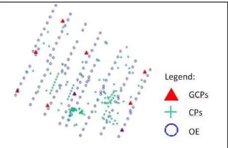
Figure 4 – Distribution of 9 GCPs for the block orientation in the a) version.
3.3 Flight at 70 m
The flight at 70 m was planned according to the same criteria as the previous flight. Given the characteristics of the camera and image scale (Table 3), the expected accuracy was fixed at 5.7
cm for σz. Figure 5 shows the overlap between the frames and the camera locations as well. In this case, unfortunately, ground level GCP were not enough available to control the solution. The photogrammetry block was oriented using 20 GCP. The statistics of RMSE of differences are shown in Table 5. The RMSE of differences shows values in X and Y comparable to the GSD and twice the GSD for the Z coordinates. The errors of CPs on building are larger than the ground level ones (especially the coordinates Y and Z are affected) as expected since in this case higher level GCP are missing. Finally the RMSE residual on all CPs is always smaller than the expected accuracy (Table 6).
Flight 140 - RMSE on the CPs
All CPs CPs on buildings CPs on the ground
Block version
# CPs DX DY DZ # CPs DX DY DZ # CPs DX DY DZ
(m) (m) (m) (m) (m) (m) (m) (m) (m)
a) 9 GCP 127 0.056 0.046 0.092 34 0.074 0.046 0.094 93 0.051 0.047 0.091 b) 28 GCP 108 0.048 0.048 0.052 34 0.055 0.043 0.064 74 0.045 0.049 0.045 c) 28+7GCP 101 0.046 0.047 0.045 27 0.051 0.041 0.053 74 0.044 0.049 0.043
Table 5 – Flight 140: coordinates difference value in the 3 configuration of UAS block on all CPs, on buildings and on the ground.
Flight 70: RMSE on the CPs
Block version
All CPs: 39 CPs on buildings (10) CPs on the ground (29)
DX DY DZ DX DY DZ DX DY DZ
(m) (m) (m) (m) (m) (m) (m) (m) (m)
20 GCP 0.021 0.047 0.056 0.022 0.111 0.086 0.020 0.021 0.049
Table 6 - Flight 70: RMSE of total CPs, of CPs on buildings and on the grounds.
Figure 5 - Image overlap and camera locations of 70 m flight.
4. DSM
4.1 Digital Surface Model production
The DSMs of both areas were created using PhotoScan as well. In this stage the level of automation of the software is quite impressive (though, for very large blocks, a huge amount of memory and processing power is required): regardless of the number of images, their spatial distribution and the shape of the object, the software executes in a fully automatic way all the 3D reconstruction procedures. If the scene depicted is 2.5D, an ad- hoc algorithm (called Height-field) grants better results with (usually) less outliers, higher processing speed and lower memory consumption. Also in this case, although, the user-manual, the scientific literature and the topics discussed in the user forum lack real information on the algorithms and techniques implemented in this stage by the software. Apparently (see for instance (PhotoScan, 2014)) except a “Fast” reconstruction method, selectable by the user before the image matching process starts, that use a multi-view approach, the depth map calculation is performed pair-wise (probably using all the possible overlapping image pairs) and merging all the results in a single 3D model.
4.2 Products & Results
Three 3D models have been produced; the first two come from the 140 m flight oriented first with 28 GCP and then with 9 GCP only; the third has been derived from the orientation of 70 m flight with 20 GCP. The validation was performed comparing the models with the GPS (grassy areas and paved surfaces) and total station (buildings) survey data.
The models were imported in ArcGis as raster, setting an interpolation resolution of 20 cm, a good compromise between maintaining the details obtained with the GSD of UAS survey and the data size.
The difference between DTM and CPs was calculated using ArcGis “Spatial Analyst Tool” that permits to interpolate the raster at the measured GPS points and extract tables of discrepancies.
For each dataset the mean and the RMS of differences were calculated. The errors were classified according to the different ground surface:
a) details: i.e. well recognizable points as road signs, manholes and tracks of playing fields (72 measured GPS points);
b) CPs on the buildings (7 survey points); c) grass field (1242 measured GPS points); d) embankment (61 measured GPS points);
e) paved roads and parking lots (2056 measured GPS points).
The results are summarized in Table 7 for the 140 m flight. As a general remark the model accuracy is not much influenced by the surface type, though one would expect the grass to be more difficult than paved surfaces; indeed at the time of the flight (November 2013) the grass cover is not as thick and dense as in spring time. The only noticeable difference is on the embankment; in these zones the residuals are larger. In fact, the tip of the pole rests on the ground and measures the terrain surface, while the photogrammetric restitution is somehow intermediate between the ground and the grass top.
Table 7 – Differences in elevation between the DSM 140 (version block with 28 GCPs and 9 GCPs) and CPs.
Comparing the results of the different block versions, in the configuration with 28 GCPs discrepancies are smaller for CPs on building and paved areas while they get worse in the grassy areas and details. Instead, there are always positive values for the DSM oriented with 28 GCPs. Considering that the differences were always calculated as DSM value minus GPS value, therefore the DSM with 9 GCPs reconstructs an elevation profile lower than those with 28 GCPs, likely inherited from the bundle adjustment.
Figure 6 – DSM of flight at 140 m and GPS survey points location.
Ground surface classification
# CPs
DSM 140m Flight 28 GCPs
DSM 140m Flight 9 GCPs
MeanDZ (m)
RMSEDZ (m)
MeanDZ (m)
RMSEDZ (m) Details 72 0.049 0.081 -0.047 0.073 CPs on
buildings 7 0.032 0.074 -0.055 0.084 Grass fields 1242 0.073 0.086 0.029 0.079 Embankment 61 0.089 0.147 0.073 0.132 Paved areas 2056 0.019 0.077 -0.057 0.084 Total 3438 0.040 0.081 -0.023 0.056
Figure 7 shows the differences between the DSM obtained for 140 m flight, using the two configuration with 28 and 9 GCP in the range between 0.2 m and -0.2 m (larger differences occur at building edges and trees, but are due to the rasterization). A global deformation between the two models is clearly visible: on the right side of the area one DSM is lower than the other, while, on the other side the two models are more on average in better agreement. This deformation isn’t related to the kind of terrain nor to its shape: in fact both sides include grassy field, paved areas and buildings. Thus different GCP distribution can introduce block deformation during the bundle adjustment.
Figure 7 – Raster at 20 cm resolution of the differences between the 140 m flight DSM with 28 GCPs (brown and azure
triangles) and 9 GCPs (in azure triangles).
For the 70 m flight less statistics were collected since the area is smaller and just one GCP configuration was considered. In addition, due to insufficient overlap (Figure 5), caused by the change of image scale, it was not possible to reconstruct the roof of the higher buildings (Figure 8). For the same reason no building top CP comparisons were performed. The comparison results for the different types of point is shown in the Table 8. Analysis of the data shows the previous behaviour: worse accuracies of grassy areas.
Table 8 – Differences between Kinematic GPS and DSM 70 with 20 GCPs.
4.3 Differences between 140 m flight and 70 m flight DSM
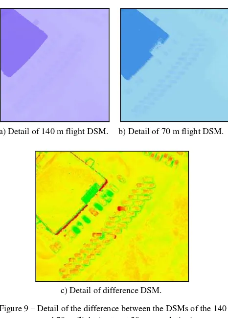
Since the 140 m flight covers also the area of the 70 m flight, a comparison has been carried out between the two DSM. Since the flights were performed at different times of the day, the difference DSM shows scene changes as well as discrepancies in unchanged areas. Figure 9 shows part of a building and a parking area in the eastern side of surveyed area: Figure 9a) and 9b) show respectively the 140 m and 70 m DSM; Figure 9c) the difference DSM. Car parked during the 140 m flight but not during the 70 m flight are green colored. When the same parking lot has been occupied by different car models in the two
flights it appears red. An inconsistency between the DSM appears in the reconstruction of the building.
Overall the differences over the whole area (not shown) are in the order of the elevation accuracy; however, areas with larger discrepancies (up to 20 cm) appear on some of the buildings.
Figure 8 – DSM of 70 m flight and GPS survey locations.
a) Detail of 140 m flight DSM. b) Detail of 70 m flight DSM.
c) Detail of difference DSM.
Figure 9 – Detail of the difference between the DSMs of the 140 m and 70 m flight (raster at 20 cm resolution).
4.4 Ortophotos
As an auxiliary product of the work two orthophotos (one for the 140 m flight and one for the 70 m) were produced with the PhotoScan tool at 10 cm resolution. Their generation has showed the problems already encountered in the generation of digital models: in particular for the higher buildings lack of reconstruction due to small overlap required manual operator intervention. These issues are particularly evident in the case of the 70 m flight, where perspective effects and sudden image DSM Flight at 70 m 20 GCPs
Ground surface
classification # CPs
MeanDZ (m)
RMSEDZ (m)
Grass fields 340 0.087 0.135
Paved areas 873 0.011 0.069
Total 1213 0.032 0.088
scale changes are larger than the other case. To solve or mitigate these problems the 140 m DSM has been used to patch up unreconstructed zones and meshed up with the 70 m DSM. Even if the planned overlap (80%) was bigger than the necessary, image scale changes weren’t managed by automatic software for feature extraction and restitution in those critic zones. On the other hand the manual restitution, which is always possible, on condition that stereo coverage is provided, is not supported by appropriate tools in the software.
In the end, as far as urban environment is concerned, where sudden and large depth changes occur, unless the flight altitude limitations imposed by the national regulation are broadened, few solutions can be used:
a) Take a greater number of frames with a shorter base; b) Take photos from different heights to maintain the same
image scale (i.e. ground and height buildings). These precautions are more expensive time consuming.
5. CONCLUSION
The paper reported an experience of UAS survey on a test area in the University Campus of Parma. Two flights at different altitude (140 and 70 m) were executed by a Falcon 8 drone; about 30 signalized ground control points were available. To validate the block orientation, 127 3D check points were measured manually on markers or on well defined features. In addition, to check the DSM, more than 3000 elevation check points were measured with GPS at ground level on different parts of the campus. Increasing the number of GCP from 9 to 28 in the 140 flight improves the accuracy, but only for the altimetric coordinates. Using GCPs also on top of buildings slightly improves the elevation accuracy. In absolute terms, the RMSE on check points is about 5 cm in all coordinates when using dense control. Since UAS surveys have normally a very small GSD and the quality of consumer-grade compact camera has greatly improved in the last few years, even few GCP (e.g. 9 GCP for a 500x500 m2 area) are enough for map update. A minimum number of GCPs to verify the reliability of the results and the absence of deformation in object space should always be provided and, due to the small size of the areas, does not substantially increase survey costs.
A DSM was generated for the 70 m flight; for the 140 m, two models (one from a block adjusted with 9 GCP and the other with 28 GCP) were generated. The validation of the 3D models performed with GPS check points measured on grassy areas and paved areas showed that for the 140 m flight the RMSE is slightly better for points on paved areas with respect to points in grass. The same applies to the 70 m flight. However, small discrepancies were found in a relative comparison between the 3D models.
Both models look fairly complete, except for parts of the roof of high rise buildings (one particularly demanding indeed). Flying at low altitude makes it difficult to handle abrupt changes in elevation due to high rise buildings (though an increase in accuracy is apparent on the planimetric coordinates). It is an operative problem that wasn’t expected during the flight planning. Ironically, the image acquisition mode of the Falcon, that is similar to that used by traditional photogrammetry, in this case might have exacerbated the problem. Indeed many UAS still shoot at the maximum frame rate allowed by the camera, providing excess images that should be later discarded or kept in the block, with an increase of the processing time.
ACKNOWLEDGEMENTS
This research is supported by the Italian Ministry of University and Research within the project “FIRB - Futuro in Ricerca 2010” – Subpixel techniques for matching, image registration and change detection (RBFR10NM3Z).
REFERENCES
Berni, J., Zarco-Tejada, P. J., Suárez, L., & Fereres, E. (2009). Thermal and narrowband multispectral remote sensing for vegetation monitoring from an unmanned aerial vehicle. Geoscience and Remote Sensing, IEEE Transactions on, 47(3), pp. 722-738.
Deseilligny, M. P., & Clery, I., 2011. Apero, an open source bundle adjustment software for automatic calibration and orientation of set of images. In Proceedings of the ISPRS Symposium 3DARCH11, Int Arch Photogramm Remote Sens Spatial Inf Sci, Vol. 38-5W16 pp. 269-277.
Eisenbeiss, H., 2009. UAS Photogrammetry. Thesis Diss. ETH No. 18515, Technische Wissenschaften ETH Zurich, IGP Mitteilung N. 105.
Gini, R., Passoni, D., Pinto, L., & Sona, G. (2012). Aerial images from an UAS system: 3d modeling and tree species classification in a park area. Int Arch Photogramm Remote Sens Spatial Inf Sci, Vol 39/B1, pp. 361-366.
González-Aguilera, D., Fernández-Hernández, J., Mancera-Taboada, J., Rodríguez-Gonzálvez, P., Hernández-López, D., Felipe-García, B., .Gozalo-Sanz, I., & Arias-Perez, B. (2012). 3D Modelling and Accuracy Assessment of Granite Quarry Using Unmanned Aerial Vehicle. ISPRS Annals of Photogrammetry, Remote Sensing and Spatial Information Sciences, Vol. 1-3, 37-42.
Kraus, K. (2007). Photogrammetry: geometry from images and laser scans. Walter de Gruyter.
Pagnano, A., Hoepf, M., Teti R., 2013, A Roadmap for Automated Power Line Inspection. Maintenance and Repair. Proc. Eighth CIRP, Volume 12, 2013, 234–239
PhotoScan, 2014. Algorithms used in Photoscan (last accessed May,9th2014)
http://www.agisoft.ru/forum/index.php?topic=89.0
Remondino, F., Del Pizzo, S., Kersten, T. P., & Troisi, S. (2012). Low-cost and open-source solutions for automated image orientation–a critical overview. In Progress in Cultural Heritage Preservation (pp. 40-54). Springer Berlin Heidelberg.
Roncella, R., Re, C., & Forlani, G. (2011). Performance evaluation of a structure and motion strategy in architecture and cultural heritage. Int. Archives of Photogrammetry, Remote Sensing and Spatial Information Sciences, 38(5/W16).
Snavely, N., Seitz, S. M., & Szeliski, R. (2006). Photo tourism: exploring photo collections in 3D. ACM transactions on graphics (TOG), 25(3), 835-846.
Ullman, S. (1979). The interpretation of structure from motion. Proceedings of the Royal Society of London. Series B. Biological Sciences, 203(1153), 405-426.