POSITIONING BASED ON INTEGRATION OF MUTI-SENSOR SYSTEMS USING
KALMAN FILTER AND LEAST SQUARE ADJUSTMENT
Mohammad Omidalizarandi *, Zhou CAO
University of Stuttgart, Dept. of Geomatics Engineering, Geschwister-Scholl-Str. 24D, 70174, Stuttgart, Germany (mohammadzarandi, zhoucao.wh )@gmail.com
KEY WORDS: Sensor fusion, Kalman Filter, Least Square Adjustment, Calibration, Dead Reckoning
ABSTRACT:
Sensor fusion is to combine different sensor data from different sources in order to make a more accurate model. In this research, different sensors (Optical Speed Sensor, Bosch Sensor, Odometer, XSENS, Silicon and GPS receiver) have been utilized to obtain different kinds of datasets to implement the multi-sensor system and comparing the accuracy of the each sensor with other sensors. The scope of this research is to estimate the current position and orientation of the Van. The Van's position can also be estimated by integrating its velocity and direction over time. To make these components work, it needs an interface that can bridge each other in a data acquisition module. The interface of this research has been developed based on using Labview software environment. Data have been transferred to PC via A/D convertor (LabJack) and make a connection to PC. In order to synchronize all the sensors, calibration parameters of each sensor is determined in preparatory step. Each sensor delivers result in a sensor specific coordinate system that contains different location on the object, different definition of coordinate axes and different dimensions and units. Different test scenarios (Straight line approach and Circle approach) with different algorithms (Kalman Filter, Least square Adjustment) have been examined and the results of the different approaches are compared together.
1. INTRODUCTION
In the current state-of-the-art, multi sensor systems play an important role in kinematic measurements and have many applications in navigation, machine guidance, mobile positioning system, monitoring and so on. Sensor fusion is to combine different sensor data from different sources in order to make a more accurate model. Positioning in the static mode is the old-fashioned and has been investigated since many years ago. However, precise positioning of the moving objects is still challenging issue and many researchers are working in this area of research. Measurement technique is so called kinematic if time is taken into account due to the movement of the object or the sensor (Foppe et al, 2004). Schwieger (2012) represents the correct definition of the real time as follow: “Real time capability means the provision of application-related results at the required point of time with the required quality”. Welsch & Heunecke (2001) defined four models (Identity model, Static model, Kinematic model and Dynamic model) to build reality with respect to geometry, time and acting forces whereas in kinematic model, time-related movements are described without consideration of acting forces. Multi sensor systems are divided in three main categories: Space-distributed systems, redundant systems and complementary systems (Schwieger, 2012). In this research, complementary system has been implemented which means different sensors acquire different measurement values to determine a target quantity. Schwieger (2008) investigated two multi sensor systems. Firstly, a high precise system which was provided by Allsat Company comprises multiple antenna Javad GNSS system and an inertial measurement unit with three vibration gyroscopes and three MEMS accelerometers. Secondly, the Modular Positioning System (MOPSY) which was developed by the Institute of Engineering Geodesy of University of Stuttgart and consisting of low cost GPS receiver in company of gyroscope, two odometers and an optical speed and distance sensor. This system has been developed based on
assumption of uniform circle drive and using the Kalman Filter approach. Schweitzer (2012) implemented multi sensor systems comprises low cost sensors (GPS ( blox ANTARIS 4), Odometer, Accelerometer (XSENS) and Gyroscope (Silicon sensing CRS05)) and then, determined the current position and orientation of the vehicle by applying extended Kalman Filter and compared the final results with PDGPS. Hong and Wang (1994) utilized a Kalman filtering approach and fuzzy to integrate sensory data. In this research, different sensors (Optical Speed Sensor, Bosch Sensor, Odometer, XSENS, Silicon and GPS receiver) have been utilized to get different kinds of datasets to implement the multi sensor systems and comparing the accuracy of the each sensor with other sensors. GPS can get the coordinates of the vehicle and the initial azimuth. The measurements of all the gyroscope sensors are rotation of the vehicle travelling and the distance which vehicle travelled during driving between each epoch. The measurement of the Optical Speed and Distance Sensor is the distance and velocity at each epoch. These sensors are attached to the Van. Bosch sensor and XSENS are sensitive sensors and should be attached to the levelled table in the centre of the gravity inside the vehicle. Therefore, XSENS, Bosch sensor and Silicon are mounted on the levelled table inside the car. Axes of Bosch sensor and XSENS must be aligned with the travel direction. Optical Speed sensor is attached to the back of the vehicle. Odometers are attached to wheels and GPS receiver is mounted on the top of the vehicle. The scope of this research is to estimate the current position and orientation of the Van. The Van equipped with a GPS unit that provides an estimate of the position and other sensors. The GPS estimate is likely to be very noisy and jump around at a high frequency, though always remaining relatively close to the real position. The Van's position can also be estimated by integrating its velocity and direction over time, determined by keeping track of the amount the accelerator is depressed and how much the steering wheel is turned. This is a technique known as dead reckoning. Typically,
dead reckoning will provide a very smooth estimate of the Van's position, but it will drift over time as small errors accumulate (Schwieger, 2009). To make these components work, it needs an interface that can bridge each other in a data acquisition module. The interface of this research has been developed based on using Labview software environment. Data have been transferred to PC via A/D convertor (LabJack) and make a connection to PC. Outputs of the most of sensors are voltage (analogue) and must be converted to the relevant unit. Therefore, it is necessary to convert analogue signals to digital signals due to making it readable for computers. In order to process at a defined point of time, real time operating system is needed. Since data request is not possible at defined point of time due to usage of operating system from resources, therefore precise synchronization has been lost. In order to synchronize all the sensors, calibration parameters of each sensor is determined in preparatory step. Knowing the exact calibration parameters of each sensor is necessary and wrong values will be affected on our analysis. In addition, synchronisation was realised by using the GPS time stamp. Each sensor delivers result in a sensor specific coordinate system that contains different location on the object, different definition of coordinate axes and different dimensions and units. In general, the Kalman Filter is used to remove disturbances caused by the measurement instruments and processes (Schweitzer, 2012). Thus, it is useful to filter raw measuring observations. In this research, different test scenarios (Straight line approach and Circle approach) with different algorithms (Kalman Filter, Least square Adjustment) have been examined and the results of the different approaches are compared together. In order to make more familiar with corresponding sensors within the multi sensor system, the brief description of them has been presented in the following sub sections.
1.1 Optical Speed and Distance Sensor
The measurement of the Optical Speed and Distance Sensor is the distance and velocity at each epoch. In this sensor, measurement principle is based on Optical correlation and raw data is Voltage (analogue).
1.2 Bosch Sensor
Measurement values of Bosch sensor are Lateral Acceleration and yaw rate. The unit of raw data is voltage (analogue) and
desired unit are and . Drive motion is in the x direction and Sensing motion is in the y direction. The z axis is the sensitive angular rate input axis (Neul et al, 2007)
Figure 1. Axis of Bosch Sensor (Neul et al, 2007)
In this project, we use this sensor to measure acceleration and rotation angle. The measurement principles are based on MEMS and Turning fork.
1.3 Odometer
In this sensor, measurement value is speed and desired unit is m/s. Data acquisition is based on counting of impulses and digital. We used this sensor for measuring rotation angle and distance. Odometer is connected directly to a driving wheel shaft. Resolution is defined by number of impulses per revolution.
1.4 XSENS
The Mti is the gyro–enhanced MEMS based Inertial Measurement Unit (IMU). Attitude and heading is referenced with gravity and the earth magnetic field. The Mti contains gyroscopes, accelerometers and magnetometers in 3D. Outputs of this sensor are 3D Orientation (360 degree), 3D acceleration, 3D rate of turn and 3D magnetic field. We connect this sensor with USB to PC. Furthermore, we can access directly to measurement values. In this project, we use this sensor to measure acceleration and rotation angle.
1.5 Silicon
In this project, we used silicon to measure rotation angle. It is robust and affordable mass-produced gyroscope for automotive and commercial customers. Angular rate sensors are used wherever rate of turn sensing is required without a fixed point of reference. The Output of this sensor is DC voltage that proportional to the rate of turn and input voltage.
1.6 GPS Receiver
The Global Positioning System (GPS) is a U.S. space-based global navigation satellite system. It provides reliable positioning, navigation, and timing services to worldwide users on a continuous basis in all weather, day and night, anywhere on or near the Earth which can observe four or more GPS satellites. GPS satellites broadcast signals from space that GPS receivers use to provide three-dimensional location (latitude, longitude, and altitude) plus precise time.
Figure 2. Sensors (a) Optical Speed and Distance Sensor, (b) Bosch Sensor, (c) Odometer, (d) XSENS, (e) Silicon, (f) GPS
Receiver
2. METHODOLOGY
Data acquisition is the process of sampling of real world physical conditions and conversion the resulting samples into digital numeric values that can be manipulated by computer for further purposes. Data acquisition system involves both hardware and software which works together to capture raw physical data into interpretable values like speed, orientation, position, etc. The data acquisition module in general consists of three parts which are as follows: data acquisition, data Processing and data storing. In this research, in order to synchronize all the sensors, calibration parameters of each sensor was determined in preparatory step. Therefore, the interface was developed using Labview software environment to transfer analogue data to PC and performing calibration. Thereafter, Matlab software has been utilized to compute the position and orientation of the vehicle based on Kalman Filter – Standard Kinematic Approach and Least Square Adjustment in straight line and circle drive. In the next sub section, development of algorithms is presented and discussed in detail.
2
s m
s
2.1 Development of algorithms
In general, typical methods and techniques to determine the trajectories are time series analysis, regression and least square adjustment as well as filter techniques, where the Kalman filter is of particular importance (Kuhlmann, 2004). The Kalman filter is essentially a set of mathematical equations that implement a predictor-corrector type estimator that is optimal in the sense and minimizing the estimated error covariance when some presumed conditions are met. The Kalman Filter can be divided into two steps: the prediction and the correction. The first step is to predict the state from the previous epoch with the dynamic model. In the second step the predicted state is corrected with the observation model, so that the error covariance of the estimator is minimized, which means the Kalman Filter is an optimal estimator. The dynamic system and the observation system are described in time domain. State vector at epoch k+1 can be predicted from the state vector at previous epoch K. Then we replace the parameter with the predicted state vector in the observation equation and we get the predicted observation. The difference between predicted observation and actual observation which is derived from our measurements is so-called innovation. Then using gain matrix K to combine the innovation with the predicted vector to get the updated state vector which fulfill the condition that the covariance of updated state vector is minimized. The advantage of the Kalman filter concept is that the computation is performed in real-time with low computational effort. The weighting of the measurement and disturbance allows a flexible adjusting of the system (Kuhlmann, 2012).
Figure 3. Real-time calculation process (Kuhlmann, 2012)
2.1.1 Kalman Filter – Standard Kinematic Approach: In this approach, the updated state vector includes 4 elements that
correspond to the coordinates of the Van at epoch k and
indicate the velocity of the Van at epoch k. (Schwieger, 2009)
(1)
Figure 4. Kalman Filter - Standard Kinematic approach (Schwieger, 2009) the predicted state vector at epoch k+1 , we need to get updated state vector at epoch k plus the time differences between epoch k+1 and epoch k in addition to velocities in both direction x and y at the epoch k. Kinematic approach is:
T
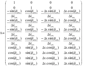
Due to independency of modular multi sensors, cofactor matrix of observations has been considered diagonal and off diagonal elements of corresponding matrix is zero. The design matrix A of the Kalman Filter - Standard Kinematic approach is:
(5)
In this algorithm, we used the acceleration from the Bosch
The Algorithm implemented within the following steps:
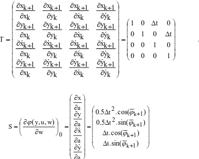
Step 1: calculating predicted state vector:
yk1T.yˆkS.w (9)
Step 2: calculating cofactor matrix of predicted state vector:
Step 3: calculating the vector of innovations:
dlk1Ak1.yk1 (11)
Where lk1: Vector of the observations
lk1: Predicted vector of observations
Step 4: calculating the cofactor matrix of innovations:
Step 5: calculating the gain matrix K:
Step 6: calculating the updated state vector (epoch k+1)
yˆk1yk1Kk1.dk1 (14)
Figure 5. Kalman filter cycle (Schweitzer, 2012)
2.1.2 Least-square Adjustment – Straight Line Approach: The general form of least square adjustment model is:
(16)
Where y = observation vector A = design matrix x = unknown vector e = error vector
Observation vector for each epoch includes following parameters:
and target quantities are as follows: , , . In order
to determine target quantities, the relationship between observation vector and unknown vector should be defined. Therefore, these relationships are determined as following models: the unknown parameters and substitution of the approximate values from above equations. Before performing derivation, equations (17) must be linearized by using Taylor expansion. Then, vector of reduced observation () is computed by subtracting vector of approximate observations ( from vector of observations ( . Thereafter, vector of reduced adjusted parameters and vector of adjusted parameters are computed respectively as follows:
(18)
This procedure is carried out in the iteration process until the pre-defined accuracy is met. After ending up the iterations, the final value of target quantities is calculated. The rest of computation includes computation of vector of residuals, cofactor matrix of adjusted observations, cofactor matrix of residuals and vector of reduced adjusted observations as follows:
(19)
2.1.3 Least Square Adjustment – Circle Approach: As the drive mode is changing from straight line to circle, it would be more accurate to utilize circle drive model of least square adjustment. This model is quite useful for significant rotation or changing direction of the driving path. In order to detect the rotation in the driving path, Bosch, Silicon and odometer sensors have been used. Then, by considering pre-defined threshold (e.g. 0.01 radian), we can distinguish straight line from circle drive and applying appropriate least square adjustment. Relationship between the parameters (x, y, ) and all the observations (X, Y, , ∆φ, ∆s) is not linear. Therefore, we have to do the linearization and set approximate values for least square Method. In this research, GPS observations have been considered as approximate values.
(20)
Figure 6. Least Square Adjustment - Circle approach (Schwieger, 2009)
3. EXPERIMENTS AND RESULTS
3.1 Kalman Filter – Standard Kinematic Approach
In order to obtain the position of trajectory, we should make an assumption for the cofactor matrix of observation. Due to special specification of each sensor and deriving better results, we considered more weights for computing rotation angle of Bosch sensor and distance from Odometer and coordinate from GPS. The values of this matrix are as follows:
,
Figure 7. Trajectory of the Vehicle – All sensors vs. GPS, Straight line (left), Circle drive (Right)
Figure 8. Displacement between GPS and modular multi sensors, Straight line (left), Circle drive (Right)
Type of drive Mean value of (m)
Mean value of (m)
Circle drive -0.2176 -0.1163
Straight line -0.0383 0.1281
Table 1. Statistical differences of different drive approaches
Figure 9. Estimated velocity of modular multi sensors vs. Optical speed and distance sensor, Straight line (left), Circle
drive (Right)
The results interpretation from this method is made base on two assumptions. In the first case study, has been considered to put more weights for rotation angle of Bosch sensor and distance from Odometer and GPS. From this considerations the displacement between GPS and calculated values are in the range 0-3 meter for circle drive scenario and 0-1.2 meter for straight line approach. In the second case study considered to increase the weight on the GPS, rotation angle of Bosch sensor and distance from Odometer. The results show that the differences with GPS trajectory become quite smaller around 0-0.4 meter both for circle drive and straight line approach. But the differences for velocity become higher comparing to the first case study.
3.2 Least-square Adjustment – Straight Line Approach
Figure 10. Trajectory of the Vehicle – All sensors vs. GPS, Straight line
Parameters Mean value Standard deviation
x axis 0.3564 (m) 0.2378 (m) y axis -0.4053 (m) 0.2589 (m) Azimuth -0.6158 (deg) 0.0063 (deg)
Table 2. Statistical differences between GPS and modular multi sensor
3.3 Least Square Adjustment – Circle Approach
In this approach, we considered rotation measurement from Odometer as the approximated azimuth to avoid sharp fluctuation of the GPS observation. This is used to improve the azimuth results as the azimuth plays an important role in our computation even more than distance measurement.
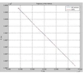
Figure 11. Trajectory of the Vehicle – All sensors vs. GPS, Circle drive
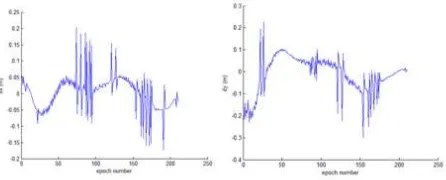
Figure 12. Displacement between GPS and adjusted values from all sensors. Differences at x-axis (left), Differences at y-axis
(right)
From figure 12, we can realise that the achieved results from this approach is much better than previous approaches. The displacement between GPS and calculated values from other sensors in x direction are in the range -0.02 – 0.02 and displacement between GPS and calculated values from other sensors in y direction are in the range -0.03 – 0.03 which seems quite good in comparison with previous approaches.
4. CONCLUSION
In this research, different test scenarios (Straight line approach and Circle approach) with different algorithms (Kalman Filter, Least square Adjustment) have been examined and the results of the different approaches are compared together. From the achieved results, we can realise that the least square adjustment for circle drive approach leads to the best result among the others. On the other hand the results from Kalman filter and least square for the other approaches is also quite reasonable and variying in decimeter until centimeter fraction. Furthermore, if we merely utilize GPS observation, the measurement of azimuth is not very accurate and that they may relate to multipath or cycle slip errors and in some cases,
leading to unexpected and truncation errors. Therefore, in this research, in order to reduce the effects of the aforementioned errors, modular multi sensor have been used and tried to obtain more accurate position and orientation of the trajectory.
Acknowledgements
The authors would like to gratefully thank the institute of engineering geodesy of University of Stuttgart for providing the test data sets of this research.
References from Journals:
Neul, R., Gomez, U.-M., Kehr, K., Bauer, W., Classen, J., Doring, C., Esch, E., Gotz, S., Hauer, J., Kuhlmann, B., Lang, C., Veith, M., Willig, R., 2007. Micromachined Angular Rate Sensors for Automotive Applications, IEEE sensors journal, Vol. 7, No. 2
References from Other Literature:
Foppe, K., Schwieger, V., Staiger, R., 2004. Grundlagen kinematischer Mess- und Auswertetechniken. In: Kinematische Messmethoden - Vermessung in Bewegung. Beiträge zum 58. DVW-Seminar am 17. und 18. Februar 2004 in Stuttgart, Wißner Verlag, Augsburg.
Hong, L. and Wang, G.-J., 1994. Integrating multisensor noisy and fuzzy data, Int. Conf. on Multi-Sensor Fusion and Integration for Intell. Syst., Las Vegas, NV, pp. 199–206.
Kuhlmann, H., 2004. Mathematische Modellbildung zu kinematischen Prozessen. In: Kinematische Messmethoden - Vermessung in Bewegung. Beiträge zum 58. DVW-Seminar am 17. und 18. Februar 2004 in Stuttgart, Wißner Verlag, Augsburg.
Kuhlmann, H., Wieland, M., 2012. Steering of a seeding process with a multi-sensor system,FIG Working Week, Rome, Italy.
Schweitzer, J., 2012. Modular Positioning using Different Motion Models. 3rd International Conference on Machine Control and Guidance, Stuttgart, Germany.
Schwieger, V., 2008. Integration of a Multiple-Antenna GNSS System and Supplementary Sensors, 1st International Conference on Machine Control & Guidance.
Schwieger, V., 2009. Terrestrial Multisensor Data Acquisition. Script of lecture within GEOENGINE master course of University Stuttgart, unpublished version 2009.
Schwieger, V., 2012. Challenges of Kinematic Measurements. FIG Working Week, Rome, Italy.
Welsch, W., Heunecke, O., 2001. Models and Terminology for the Analysis of Geodetic Monitoring Observations. FIG Publication, Ad-Hoc Committee of FIG Working Group 6.1.
References from websites: http://www.xsens.com/en/general/mti