The Path to Predictive Analytics and
Machine Learning
The Path to Predictive Analytics and Machine Learning by Conor Doherty, Steven Camiña, Kevin White, and Gary Orenstein Copyright © 2017 O’Reilly Media Inc. All rights reserved.
Printed in the United States of America.
Published by O’Reilly Media, Inc., 1005 Gravenstein Highway North, Sebastopol, CA 95472. O’Reilly books may be purchased for educational, business, or sales promotional use. Online editions are also available for most titles (http://safaribooksonline.com). For more information, contact our corporate/institutional sales department: 800-998-9938 or [email protected].
Editors: Tim McGovern and
The O’Reilly logo is a registered trademark of O’Reilly Media, Inc. The Path to Predictive Analytics and Machine Learning, the cover image, and related trade dress are trademarks of O’Reilly Media, Inc.
While the publisher and the authors have used good faith efforts to ensure that the information and instructions contained in this work are accurate, the publisher and the authors disclaim all
responsibility for errors or omissions, including without limitation responsibility for damages
resulting from the use of or reliance on this work. Use of the information and instructions contained in this work is at your own risk. If any code samples or other technology this work contains or describes is subject to open source licenses or the intellectual property rights of others, it is your responsibility to ensure that your use thereof complies with such licenses and/or rights.
Introduction
An Anthropological Perspective
If you believe that as a species, communication advanced our evolution and position, let us take a quick look from cave paintings, to scrolls, to the printing press, to the modern day data storage industry.
Marked by the invention of disk drives in the 1950s, data storage advanced information sharing broadly. We could now record, copy, and share bits of information digitally. From there emerged superior CPUs, more powerful networks, the Internet, and a dizzying array of connected devices. Today, every piece of digital technology is constantly sharing, processing, analyzing, discovering, and propagating an endless stream of zeros and ones. This web of devices tells us more about ourselves and each other than ever before.
Of course, to meet these information sharing developments, we need tools across the board to help. Faster devices, faster networks, faster central processing, and software to help us discover and harness new opportunities.
Often, it will be fine to wait an hour, a day, even sometimes a week, for the information that enriches our digital lives. But more frequently, it’s becoming imperative to operate in the now.
In late 2014, we saw emerging interest and adoption of multiple in-memory, distributed architectures to build real-time data pipelines. In particular, the adoption of a message queue like Kafka,
transformation engines like Spark, and persistent databases like MemSQL opened up a new world of capabilities for fast business to understand real-time data and adapt instantly.
This pattern led us to document the trend of real-time analytics in our first book, Building Real-Time Data Pipelines: Unifying Applications and Analytics with In-Memory Architectures (O’Reilly, 2015). There, we covered the emergence of in-memory architectures, the playbook for building real-time pipelines, and best practices for deployment.
Since then, the world’s fastest companies have pushed these architectures even further with machine learning and predictive analytics. In this book, we aim to share this next step of the real-time analytics journey.
Chapter 1. Building Real-Time Data
Pipelines
Discussions of predictive analytics and machine learning often gloss over the details of a difficult but crucial component of success in business: implementation. The ability to use machine learning models in production is what separates revenue generation and cost savings from mere intellectual novelty. In addition to providing an overview of the theoretical foundations of machine learning, this book
discusses pragmatic concerns related to building and deploying scalable, production-ready machine learning applications. There is a heavy focus on real-time uses cases including both operational
applications, for which a machine learning model is used to automate a decision-making process, and
interactive applications, for which machine learning informs a decision made by a human.
Given the focus of this book on implementing and deploying predictive analytics applications, it is important to establish context around the technologies and architectures that will be used in
production. In addition to the theoretical advantages and limitations of particular techniques, business decision makers need an understanding of the systems in which machine learning applications will be deployed. The interactive tools used by data scientists to develop models, including domain-specific languages like R, in general do not suit low-latency production environments. Deploying models in production forces businesses to consider factors like model training latency, prediction (or “scoring”) latency, and whether particular algorithms can be made to run in distributed data processing
environments.
Before discussing particular machine learning techniques, the first few chapters of this book will examine modern data processing architectures and the leading technologies available for data processing, analysis, and visualization. These topics are discussed in greater depth in a prior book (Building Real-Time Data Pipelines: Unifying Applications and Analytics with In-Memory Architectures [O’Reilly, 2015]); however, the overview provided in the following chapters offers sufficient background to understand the rest of the book.
Modern Technologies for Going Real-Time
To build real-time data pipelines, we need infrastructure and technologies that accommodate ultrafast data capture and processing. Real-time technologies share the following characteristics: 1)
Figure 1-1. Characteristics of real-time technologies
High-Throughput Messaging Systems
Many real-time data pipelines begin with capturing data at its source and using a high-throughput messaging system to ensure that every data point is recorded in its right place. Data can come from a wide range of sources, including logging information, web events, sensor data, financial market streams, and mobile applications. From there it is written to file systems, object stores, and databases.
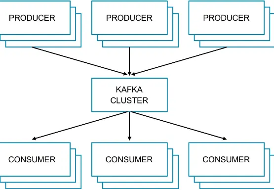
Apache Kafka is an example of a high-throughput, distributed messaging system and is widely used across many industries. According to the Apache Kafka website, “Kafka is a distributed, partitioned, replicated commit log service.” Kafka acts as a broker between producers (processes that publish their records to a topic) and consumers (processes that subscribe to one or more topics). Kafka can handle terabytes of messages without performance impact. This process is outlined in Figure 1-2.
Because of its distributed characteristics, Kafka is built to scale producers and consumers with ease by simply adding servers to the cluster. Kafka’s effective use of memory, combined with a commit log on disk, provides ideal performance for real-time pipelines and durability in the event of server failure.
With our message queue in place, we can move to the next piece of data pipelines: the transformation tier.
Data Transformation
The data transformation tier takes raw data, processes it, and outputs the data in a format more
conducive to analysis. Transformers serve a number of purposes including data enrichment, filtering, and aggregation.
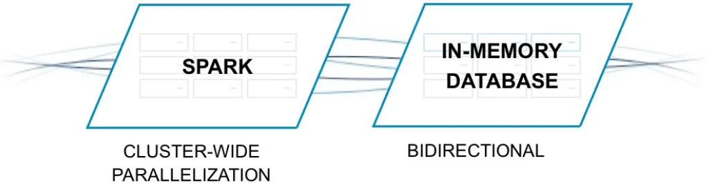
Apache Spark is often used for data transformation (see Figure 1-3). Like Kafka, Spark is a distributed, memory-optimized system that is ideal for real-time use cases. Spark also includes a streaming library and a set of programming interfaces to make data processing and transformation easier.
Figure 1-3. Spark data processing framework
When building real-time data pipelines, Spark can be used to extract data from Kafka, filter down to a smaller dataset, run enrichment operations, augment data, and then push that refined dataset to a
Figure 1-4. High-throughput connectivity between an in-memory database and Spark
Persistent Datastore
To analyze both real-time and historical data, it must be maintained beyond the streaming and
transformations layers of our pipeline, and into a permanent datastore. Although unstructured systems like Hadoop Distributed File System (HDFS) or Amazon S3 can be used for historical data
persistence, neither offer the performance required for real-time analytics.
On the other hand, a memory-optimized database can provide persistence for real-time and historical data as well as the ability to query both in a single system. By combining transactions and analytics in a memory-optimized system, data can be rapidly ingested from our transformation tier and held in a datastore. This allows applications to be built on top of an operational database that supplies the application with the most recent data available.
Moving from Data Silos to Real-Time Data Pipelines
In a world in which users expect tailored content, short load times, and up-to-date information, building real-time applications at scale on legacy data processing systems is not possible. This is because traditional data architectures are siloed, using an Online Transaction Processing (OLTP)-optimized database for operational data processing and a separate Online Analytical Processing (OLAP)-optimized data warehouse for analytics.
The Enterprise Architecture Gap
Figure 1-5. Legacy data processing model
OLAP silo
OLAP-optimized data warehouses cannot handle one-off inserts and updates. Instead, data must be organized and loaded all at once—as a large batch—which results in an offline operation that runs overnight or during off-hours. The tradeoff with this approach is that streaming data cannot be queried by the analytical database until a batch load runs. With such an architecture, standing up a real-time application or enabling analyst to query your freshest dataset cannot be achieved.
OLTP silo
On the other hand, an OLTP database typically can handle high-throughput transactions, but is not able to simultaneously run analytical queries. This is especially true for OLTP databases that use disk as a primary storage medium, because they cannot handle mixed OLTP/OLAP workloads at scale.
The fundamental flaw in a batch processing system can be illustrated through an example of any real-time application. For instance, if we take a digital advertising application that combines user
attributes and click history to serve optimized display ads before a web page loads, it’s easy to spot where the siloed model breaks. As long as data remains siloed in two systems, it will not be able to meet Service-Level Agreements (SLAs) required for any real-time application.
Real-Time Pipelines and Converged Processing
Businesses implement real-time data pipelines in many ways, and each pipeline can look different depending on the type of data, workload, and processing architecture. However, all real-time pipelines follow these fundamental principles:
Data must be processed and transformed on-the-fly so that it is immediately available for querying when it reaches a persistent datastore
An operational datastore must be able to run analytics with low latency The system of record must be converged with the system of insight
One common example of a real-time pipeline configuration can be found using the technologies
Chapter 2. Processing Transactions and
Analytics in a Single Database
Historically, businesses have separated operations from analytics both conceptually and practically. Although every large company likely employs one or more “operations analysts,” generally these individuals produce reports and recommendations to be implemented by others, in future weeks and months, to optimize business operations. For instance, an analyst at a shipping company might detect trends correlating to departure time and total travel times. The analyst might offer the recommendation that the business should shift its delivery schedule forward by an hour to avoid traffic. To borrow a term from computer science, this kind of analysis occurs asynchronously relative to day-to-day operations. If the analyst calls in sick one day before finishing her report, the trucks still hit the road and the deliveries still happen at the normal time. What happens in the warehouses and on the roads that day is not tied to the outcome of any predictive model. It is not until someone reads the analyst’s report and issues a company-wide memo that deliveries are to start one hour earlier that the results of the analysis trickle down to day-to-day operations.
Legacy data processing paradigms further entrench this separation between operations and analytics. Historically, limitations in both software and hardware necessitated the separation of transaction processing (INSERTs, UPDATEs, and DELETEs) from analytical data processing (queries that return some interpretable result without changing the underlying data). As the rest of this chapter will discuss, modern data processing frameworks take advantage of distributed architectures and in-memory storage to enable the convergence of transactions and analytics.
To further motivate this discussion, envision a shipping network in which the schedules and routes are determined programmatically by using predictive models. The models might take weather and traffic data and combine them with past shipping logs to predict the time and route that will result in the most efficient delivery. In this case, day-to-day operations are contingent on the results of analytic predictive models. This kind of on-the-fly automated optimization is not possible when transactions and analytics happen in separate siloes.
Hybrid Data Processing Requirements
For a database management system to meet the requirements for converged transactional and analytical processing, the following criteria must be met:
Memory optimized
input/output (I/O) required for real-time operations. Access to real-time and historical data
Converging OLTP and OLAP systems requires the ability to compare real-time data to statistical models and aggregations of historical data. To do so, our database must accommodate two types of workloads: high-throughput operational transactions, and fast analytical queries.
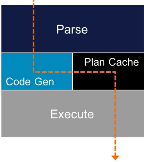
Compiled query execution plans
By eliminating disk I/O, queries execute so rapidly that dynamic SQL interpretation can become a bottleneck. To tackle this, some databases use a caching layer on top of their Relational Database Management System (RDBMS). However, this leads to cache invalidation issues that result in minimal, if any, performance benefit. Executing a query directly in memory is a better approach because it maintains query performance (see Figure 2-1).
Figure 2-1. Compiled query execution plans
Multiversion concurrency control
Reaching the high-throughput necessary for a hybrid, real-time engine can be achieved through lock-free data structures and multiversion concurrency control (MVCC). MVCC enables data to be accessed simultaneously, avoiding locking on both reads and writes.
Fault tolerance and ACID compliance
With each of the aforementioned technology requirements in place, transactions and analytics can be consolidated into a single system built for real-time performance. Moving to a hybrid database architecture opens doors to untapped insights and new business opportunities.
Benefits of a Hybrid Data System
For data-centric organizations, a single engine to process transactions and analytics results in new sources of revenue and a simplified computing structure that reduces costs and administrative overhead.
New Sources of Revenue
Achieving true “real-time” analytics is very different from incrementally faster response times.
Analytics that capture the value of data before it reaches a specified time threshold—often a fraction of a second—and can have a huge impact on top-line revenue.
An example of this can be illustrated in the financial services sector. Financial investors and analyst must be able to respond to market volatility in an instant. Any delay is money out of their pockets. Limitations with OLTP to OLAP batch processing do not allow financial organizations to respond to fluctuating market conditions as they happen. A single database approach provides more value to investors every second because they can respond to market swings in an instant.
Reducing Administrative and Development Overhead
By converging transactions and analytics, data no longer needs to move from an operational database to a siloed data warehouse to deliver insights. This gives data analysts and administrators more time to concentrate efforts on business strategy, as ETL often takes hours to days.
When speaking of in-memory computing, questions of data persistence and high availability always arise. The upcoming section dives into the details of in-memory, distributed, relational database systems and how they can be designed to guarantee data durability and high availability.
Data Persistence and Availability
By definition an operational database must have the ability to store information durably with resistance to unexpected machine failures. More specifically, an operational database must do the following:
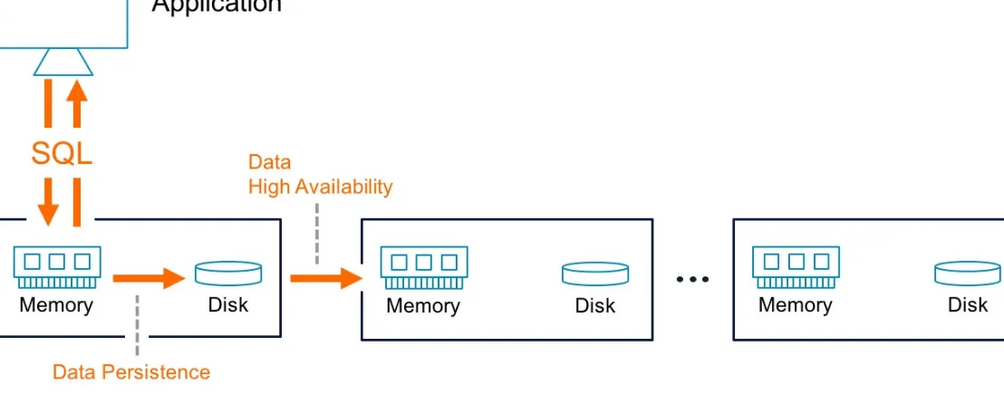
Save all of its information to disk storage for durability
Ensure that the data is highly available by maintaining a readily accessible second copy of all data, and automatically fail-over without downtime in case of server crashes
Figure 2-2. In-memory database persistence and high availability
Data Durability
For data storage to be durable, it must survive any server failures. After a failure, data should also be recoverable into a transactionally consistent state without loss or corruption to data.
Any well-designed in-memory database will guarantee durability by periodically flushing snapshots from the in-memory store into a durable disk-based copy. Upon a server restart, an in-memory
database should also maintain transaction logs and replay snapshot and transaction logs. This is illustrated through the following scenario:
Suppose that an application inserts a new record into a database. The following events will occur as soon as a commit is issued:
1. The inserted record will be written to the datastore in-memory.
2. A log of the transaction will be stored in a transaction log buffer in memory. 3. When the transaction log buffer is filled, its contents are flushed to disk.
The size of the transaction log buffer is configurable, so if it is set to 0, the transaction log will be flushed to disk after each committed transaction.
4. Periodically, full snapshots of the database are taken and written to disk.
The number of snapshots to keep on disk and the size of the transaction log at which a snapshot is taken are configurable. Reasonable defaults are typically set.
An ideal database engine will include numerous settings to control data persistence, and will allow a user the flexibility to configure the engine to support full persistence to disk or no durability at all.
Data Availability
For the most part, in a multimachine system, it’s acceptable for data to be lost in one machine, as long as data is persisted elsewhere in the system. Upon querying the data, it should still return a
transactionally consistent result. This is where high availability enters the equation. For data to be highly available, it must be queryable from a system regardless of failures from some machines within a system.
This is better illustrated by using an example from a distributed system, in which any number of machines can fail. If failure occurs, the following should happen:
1. The machine is marked as failed throughout the system.
2. A second copy of data in the failed machine, already existing in another machine, is promoted to be the “master” copy of data.
3. The entire system fails over to the new “master” data copy, removing any system reliance on data present in the failed system.
4. The system remains online (i.e., queryable) throughout the machine failure and data failover times. 5. If the failed machine recovers, the machine is integrated back into the system.
A distributed database system that guarantees high availability must also have mechanisms for
maintaining at least two copies of data at all times. Distributed systems should also be robust, so that failures of different components are mostly recoverable, and machines are reintroduced efficiently and without loss of service. Finally, distributed systems should facilitate cross-datacenter replication, allowing for data replication across wide distances, often times to a disaster recovery center offsite.
Data Backup
Chapter 3. Dawn of the Real-Time
Dashboard
Before delving further into the systems and techniques that power predictive analytics applications, human consumption of analytics merits further discussion. Although this book focuses largely on applications using machine learning models to make decisions autonomously, we cannot forget that it is ultimately humans designing, building, evaluating, and maintaining these applications. In fact, the emergence of this type of application only increases the need for trained data scientists capable of understanding, interpreting, and communicating how and how well a predictive analytics application works.
Moreover, despite this book’s emphasis on operational applications, more traditional human-centric, report-oriented analytics will not go away. If anything, its value will only increase as data processing technology improves, enabling faster and more sophisticated reporting. Improvements like reduced Extract, Transform, and Load (ETL) latency and faster query execution empowers data scientists and increases the impact they can have in an organization.
Data visualization is arguably the single most powerful method for enabling humans to understand and spot patterns in a dataset. No one can look at a spreadsheet with thousands or millions of rows and make sense of it. Even the results of a database query, meant to summarize characteristics of the dataset through aggregation, can be difficult to parse when it is just lines and lines of numbers. Moreover, visualizations are often the best and sometimes only way to communicate findings to a nontechnical audience.
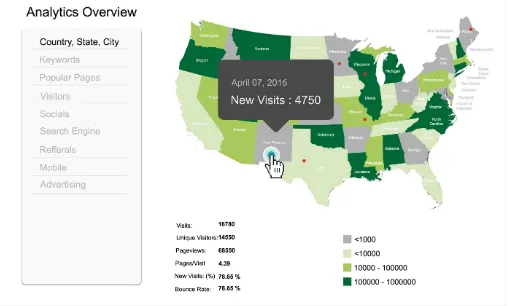
Business Intelligence (BI) software enables analysts to pull data from multiple sources, aggregate the data, and build custom visualizations while writing little or no code. These tools come with templates that allow analysts to create sophisticated, even interactive, visualization without being expert
Figure 3-1. Sample geographic visualization dashboard
Other related visualizations for an online retail site could be a bar chart that shows the distribution of web activity throughout the different hours of each day, or a pie chart that shows the categories of products purchased on the site over a given time period.
Historically, out-of-the-box visual BI dashboards have been optimized for data warehouse
technologies. Data warehouses typically require complex ETL jobs that load data from real-time systems, thus creating latency between when events happen and when information is available and actionable. As described in the last chapters, technology has progressed—there are now modern databases capable of ingesting large amounts of data and making that data immediately actionable without the need for complex ETL jobs. Furthermore, visual dashboards exist in the market that accommodate interoperability with real-time databases.
Choosing a BI Dashboard
Choosing a BI dashboard must be done carefully depending on existing requirements in your enterprise. This section will not make specific vendor recommendations, but it will cite several examples of real-time dashboards.
Real-time dashboards allow instantaneous queries to the underlying data source
Dashboards that are designed to be time must be able to query underlying sources in real-time, without needing to cache any data. Historically, dashboards have been optimized for data warehouse solutions, which take a long time to query. To get around this limitation, several BI dashboards store or cache information in the visual frontend as a performance optimization, thus sacrificing real-time in exchange for performance.
Real-time dashboards are easily and instantly shareable
Real-time dashboards facilitate real-time decision making, which is enabled by how fast knowledge or insights from the visual dashboard can be shared to a larger group to validate a decision or gather consensus. Hence, real-time dashboards must be easily and instantaneously shareable; ideally hosted on a public website that allows key stakeholders to access the
visualization.
Real-time dashboards are easily customizable and intuitive
Customizable and intuitive dashboards are a basic requirement for all good BI dashboards, and this condition is even more important for real-time dashboards. The easier it is to build and modify a visual dashboard, the faster it would be to take action and make decisions.
Real-Time Dashboard Examples
The rest of this chapter will dive into more detail around modern dashboards that provide real-time capabilities out of the box. Note that the vendors described here do not represent the full set of BI dashboards in the market. The point here is to inform you of possible solutions that you can adopt within your enterprise. The aim of describing the following dashboards is not to recommend one over the other. Building custom dashboards will be covered later in this chapter.
Tableau
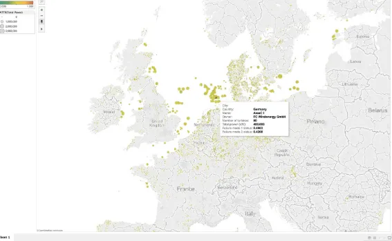
As far as BI dashboard vendors are concerned, Tableau has among the largest market share in the industry. Tableau has a desktop version and a server version that either your company can host or Tableau can host for you (i.e., Tableau Online). Tableau can connect to real-time databases such as MemSQL with an out-of-the-box connector or using the MySQL protocol connector. Figure 3-2
Figure 3-2. Tableau dashboard showing geographic distribution of wind farms in Europe
Zoomdata
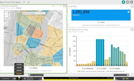
Among the examples given in this chapter, Zoomdata facilitates real-time visualization most
Figure 3-3. Zoomdata dashboard showing taxi trip information in New York City
Looker
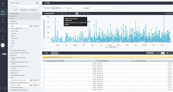
Looker is another powerful BI tool that helps you to create real-time dashboards with ease. Looker also utilizes its own custom language, called LookML, for describing dimensions, fields, aggregates and relationships in a SQL database. The Looker app uses a model written in LookML to construct SQL queries against SQL databases, like MemSQL. Figure 3-4 is an example of an exploratory visualization of orders in an online retail store.
Figure 3-4. Looker dashboard showing a visualization of orders in an online retail store
Building Custom Real-Time Dashboards
Although out-of-the-box BI dashboards provide a lot of functionality and flexibility for building visual dashboards, they do not necessarily provide the required performance or specific visual
features needed for your enterprise use case. Furthermore, these dashboards are also separate pieces of software, incurring extra cost and requiring you to work with a third-party vendor to support the technology. For specific real-time analysis use cases for which you know exactly what information to extract and visualize from your real-time data pipeline, it is often faster and cheaper to build a custom real-time dashboard in-house instead of relying on a third-party vendor.
Database Requirements for Real-Time Dashboards
Building a custom visual dashboard on top of a real-time database requires that the database have the characteristics detailed in the following subsections.
Support for various programming languages
The choice of which programming language to use for a custom real-time dashboard is at the
discretion of the developers. There is no “proper” programming language or protocol that is best for developing custom real-time dashboards. It is recommended to go with what your developers are familiar with, and what your enterprise has access to. For example, several modern custom real-time dashboards are designed to be opened in a web browser, with the dashboard itself built with a
communicating with a performant relational database.
All real-time databases must provide clear interfaces through which the custom dashboard can
interact. The best programmatic interfaces are those based on known standards, and those that already provide native support for a variety of programming languages. A good example of such an interface is SQL. SQL is a known standard with a variety of interfaces for popular programming languages— Java, C, Python, Ruby, Go, PHP, and more. Relational databases (full SQL databases) facilitate easy building of custom dashboards by allowing the dashboards to be created using almost any
programming language.
Fast data retrieval
Good visual real-time dashboards require fast data retrieval in addition to fast data ingest. When building real-time data pipelines, the focus tends to be on the latter, but for real-time data visual dashboards, the focus is on the former. There are several databases that have very good data ingest rates but poor data retrieval rates. Good real-time databases have both. A real-time dashboard is only as “real-time” as the speed that it can render its data, which is a function of how fast the data can be retrieved from the underlying database. It also should be noted that visual dashboards are typically interactive, which means the viewer should be able to click or drill down into certain aspects of the visualizations. Drilling down typically requires retrieving more data from the database each time an action is taken on the dashboard’s user interface. For those clicks to return quickly, data must be retrieved quickly from the underlying database.
Ability to combine separate datasets in the database
Building a custom visual dashboard might require combining information of different types coming from different sources. Good real-time databases should support this. For example, consider building a custom real-time visual dashboard from an online commerce website that captures information about the products sold, customer reviews, and user navigation clicks. The visual dashboard built for this can contain several charts—one for popular products sold, another for top customers, and one for the top reviewed products based on customer reviews. The dashboard must be able to join these separate datasets. This data joining can happen within the underlying database or in the visual dashboard. For the sake of performance, it is better to join within the underlying database. If the database is unable to join data before sending it to the custom dashboard, the burden of performing the join will fall to the dashboard application, which leads to sluggish performance.
Ability to store real-time and historical datasets
Chapter 4. Redeploying Batch Models in
Real Time
For all the greenfield opportunities to apply machine learning to business problems, chances are your organization already uses some form of predictive analytics. As mentioned in previous chapters, traditionally analytical computing has been batch oriented in order to work around the limitations of ETL pipelines and data warehouses that are not designed for real-time processing. In this chapter, we take a look at opportunities to apply machine learning to real-time problems by repurposing existing models.
Future opportunities for machine learning and predictive analytics span infinite possibilities, but there is still an incredible amount of easily accessible opportunities today. These come by applying
existing batch processes based on statistical models to real-time data pipelines. The good news is that there are straightforward ways to accomplish this that quickly put the business rapidly ahead. Even for circumstances in which batch processes cannot be eliminated entirely, simple improvements to architectures and data processing pipelines can drastically reduce latency and enable businesses to update predictive models more frequently and with larger training datasets.
Batch Approaches to Machine Learning
Historically, machine learning approaches were often constrained to batch processing. This resulted from the amount of data required for successful modeling, and the restricted performance of
traditional systems.
Figure 4-1. Batch approach to machine learning
With the advent of distributed systems, initial constraints were removed. For example, the Hadoop Distributed File System (HDFS) provided a plentiful approach to low-cost storage. New scalable streaming and database technologies provided the ability to process and serve data in real time. Coupling these systems together provides both a real-time and batch architecture.
This approach is often referred to as a Lambda architecture. A Lambda architecture often consists of three layer: a speed layer, a batch layer, and a serving layer, as illustrated in Figure 4-2.
The advantage to Lambda is a comprehensive approach to batch and real-time workflows. The disadvantage is that maintaining two pipelines can lead to excessive management and administration to achieve effective results.
Figure 4-2. Lambda architecture
Although not every application requires real-time data, virtually every industry requires real-time solutions. For example, in real estate, transactions do not necessarily need to be logged to the millisecond. However, when every real estate transaction is logged to a database, and a company wants to provide ad hoc access to that data, a real-time solution is likely required.
Other areas for machine learning and predictive analytics applications include the following: Information assets
Let’s take a look at manufacturing as just one example.
Manufacturing Example
Manufacturing is often a high-stakes, high–capital investment, high-scale production operation. We see this across mega-industries including automotive, electronics, energy, chemicals, engineering, food, aerospace, and pharmaceuticals.
Companies will frequently collect high-volume sensor data from sources such as these: Manufacturing equipment
Robotics
Process measurements Energy rigs
Construction equipment
The sensor information provides readings on the health and efficiency of the assets, and is critical in areas of high capital expenditure combined with high operational expenditure.
Let’s consider the application of an energy rig. With drill bit and rig costs ranging in the millions, making use of these assets efficiently is paramount.
Original Batch Approach
assist in determining the best approach.
Traditional pipelines involve collecting drill bit information and sending that through a traditional enterprise message bus, overnight batch processing, and guidance for the next day’s operations. Companies frequently rely on statistical modeling software from companies like SAS to provide analytics on sensor information. Figure 4-3 offers an example of an original batch approach.
Figure 4-3. Original batch approach
Real-Time Approach
To improve operations, energy companies seek easier facilitation of adding and adjusting new data pipelines. They also desire the ability to process both real-time and historical data within a single system to avoid ETL, and they want real-time scoring of existing models.
Figure 4-4. Real-time data pipeline supported by Kafka, Spark, and in-memory database
Technical Integration and Real-Time Scoring
The new real-time solution begins with the same sensor inputs. Typically, the software for edge sensor monitoring can be directed to feed sensor information to Kafka.
After the data is in Kafka, it is passed to Spark for transformation and scoring. This step is the crux of the pipeline. Spark enables the scoring by running incoming data through existing models.
In this example, an SAS model can be exported as Predictive Model Markup Language (PMML) and embedded inside the pipeline as part of a Java Archive (JAR) file.
After the data has been scored, both the raw sensor data and the results of the model on that data are saved in the database in the same table.
When real-time scoring information is colocated with the sensor data, it becomes immediately available for query without the need for precomputing or batch processing.
Immediate Benefits from Batch to Real-Time Learning
section:
Consistency with existing models
By using existing models and bringing them into a real-time workflow, companies can maintain consistency of modeling.
Speed to production
Using existing models means more rapid deployment and an existing knowledge base around those models.
Immediate familiarity with real-time streaming and analytics
By not changing models, but changing the speed, companies can get immediate familiarity with modern data pipelines.
Harness the power of distributed systems
Pipelines built with Kafka, Spark, and MemSQL harness the power of distributed systems and let companies benefit from the flexibility and performance of such systems. For example, companies can use readily available industry standard servers, or cloud instances to stand up new data pipelines.
Cost savings
Most important, these real-time pipelines facilitate dramatic cost savings. In the case of energy drilling, companies need to determine the health and efficiency of the drilling operation. Push a drill bit too far and it will break, costing millions to replace and lost time for the overall rig. Retire a drill bit too early and money is left on the table. Going to a real-time model lets
Chapter 5. Applied Introduction to Machine
Learning
Even though the forefront of artificial intelligence research captures headlines and our imaginations, do not let the esoteric reputation of machine learning distract from the full range of techniques with practical business applications. In fact, the power of machine learning has never been more
accessible. Whereas some especially oblique problems require complex solutions, often, simpler methods can solve immediate business needs, and simultaneously offer additional advantages like faster training and scoring. Choosing the proper machine learning technique requires evaluating a series of tradeoffs like training and scoring latency, bias and variance, and in some cases accuracy versus complexity.
This chapter provides a broad introduction to applied machine learning with emphasis on resolving these tradeoffs with business objectives in mind. We present a conceptual overview of the theory underpinning machine learning. Later chapters will expand the discussion to include system design considerations and practical advice for implementing predictive analytics applications. Given the experimental nature of applied data science, the theme of flexibility will show up many times. In addition to the theoretical, computational, and mathematical features of machine learning techniques, the reality of running a business with limited resources, especially limited time, affects how you should choose and deploy strategies.
Before delving into the theory behind machine learning, we will discuss the problem it is meant to solve: enabling machines to make decisions informed by data, where the machine has “learned” to perform some task through exposure to training data. The main abstraction underpinning machine learning is the notion of a model, which is a program that takes an input data point and then outputs a prediction.
There are many types of machine learning models and each formulates predictions differently. This and subsequent chapters will focus primarily on two categories of techniques: supervised and unsupervised learning.
Supervised Learning
The distinguishing feature of supervised learning is that the training data is labeled. This means that, for every record in the training dataset, there are both features and a label. Features are the data representing observed measurements. Labels are either categories (in a classification model) or values in some continuous output space (in a regression model). Every record associates with some outcome.
other meteorological information and then output a prediction about the probability of rain. A regression model might output a prediction or “score” representing estimated inches of rain. A classification model might output a prediction as “precipitation” or “no precipitation.” Figure 5-1
depicts the two stages of supervised learning.
Figure 5-1. Training and scoring phases of supervised learning
“Supervised” refers to the fact that features in training data correspond to some observed outcome. Note that “supervised” does not refer to, and certainly does not guarantee, any degree of data quality. In supervised learning, as in any area of data science, discerning data quality—and separating signal from noise—is as critical as any other part of the process. By interpreting the results of a query or predictions from a model, you make assumptions about the quality of the data. Being aware of the assumptions you make is crucial to producing confidence in your conclusions.
Regression
Regression models are supervised learning models that output results as a value in a continuous prediction space (as opposed to a classification model, which has a discrete output space). The solution to a regression problem is the function that best approximates the relationship between features and outcomes, where “best” is measured according to an error function. The standard error measurement function is simply Euclidian distance—in short, how far apart are the predicted and actual outcomes?
Regression models will never perfectly fit real-world data. In fact, error measurements approaching zero usually points to overfitting, which means the model does not account for “noise” or variance in the data. Underfitting occurs when there is too much bias in the model, meaning flawed assumptions prevent the model from accurately learning relationships between features and outputs.
Figure 5-2. Examples of linear and polynomial regression
Figure 5-3. Linear regression in two dimensions
There are many types of regression and layers of categorization—this is true of many machine
following form:
a x + a x + … + a x + b
One advantage of linear models is the ease of scoring. Even in high dimensions—when there are several features—scoring consists of just scalar addition and multiplication. Other regression techniques give a solution as a polynomial or a logistic function. The following table describes the characteristics of different forms of regression.
Regression
model Solution in two dimensions Output space
Linear ax + b Continuous
Polynomial a x + a x + … + a x + a + a Continuous
Logistic L/(1 + e ) Continuous (e.g., population modeling) or discrete (binary categoricalresponse)
It is also useful to categorize regression techniques by how they measure error. The format of the solution—linear, polynomial, logistic—does not completely characterize the regression technique. In fact, different error measurement functions can result in different solutions, even if the solutions take the same form. For instance, you could compute multiple linear regressions with different error measurement functions. Each regression will yield a linear solution, but the solutions can have different slopes or intercepts depending on error function.
The method of least squares is the most common technique for measuring error. In least-squares approaches, you compute the total error as the sum of squares of the errors the solution relative to each record in the training data. The “best fit” is the function that minimizes the sum of squared errors. Figure 5-4 is a scatterplot and regression function, with red lines drawn in representing the prediction error for a given point. Recall that the error is the distance between the predicted outcome and the actual outcome. The solution with the “best fit” is the one that minimizes the sum of each error squared.
1 1 2 2 n–1 n–1
1 n 2 n–1 n n n
+ 1
Figure 5-4. A linear regression, with red lines representing prediction error for a given training data point
Least squares is commonly associated with linear regression. In particular, a technique called Ordinary Least Squares is a common way of finding the regression solution with the best fit. However, least-squares techniques can be used with polynomial regression, as well. Whether the regression solution is linear or a higher degree polynomial, least squares is simply a method of measuring error. The format of the solution, linear or polynomial, determines what shape you are trying to fit to the data. However, in either case, the problem is still finding the prediction function that minimizes error over the training dataset.
Although Ordinary Least Squares provides a strong intuition for what the error measurement function represents, there are many ways of defining error in a regression problem. There are many variants on least-squares error function, such as weighted least squares, in which some observations are given more or less weight according to some metric that assesses data quality. There are also various approaches that fall under regularization, which is a family of techniques used to make solutions more generalizable rather than overfit to a particular training set. Popular techniques for regularized least squares includes Ridge Regression and LASSO.
features and outcomes of a dataset, and variance, which is naturally occurring “noise” in a dataset. Too much bias in the model causes underfitting, whereas too much variance causes overfitting. Bias and variance tend to inversely correlate—when one goes up the other goes down—which is why data scientists talk about a “bias-variance tradeoff.” Well-fit models find a balance between the two
sources of error.
Classification
Classification is very similar to regression and uses many of the same underlying techniques. The main difference is the format of the prediction. The intuition for regression is that you’re matching a line/plane/surface to approximate some trend in a dataset, and every combination of features
corresponds to some point on that surface. Formulating a prediction is a matter of looking at the score at a given point. Binary classification is similar, except instead of predicting by using a point on the surface, it predicts one of two categories based on where the point resides relative to the surface (above or below). Figure 5-5 shows a simple example of a linear binary classifier.
Figure 5-5. Linear binary classifier
for training both regression and classification models.
There are also “multiclass” classifiers, which can use more than two categories. A classic example of a multiclass classifier is a handwriting recognition program, which must analyze every character and then classify what letter, number, or symbol it represents.
Unsupervised Learning
The distinguishing feature of unsupervised learning is that data is unlabeled. This means that there are no outcomes, scores, or categorizations associated with features in training data. As with supervised learning, “unsupervised” does not refer to data quality. As in any area of data science, training data for unsupervised learning will not be perfect, and separating signal from noise is a crucial component of training a model.
The purpose of unsupervised learning is to discern patterns in data that are not known beforehand. One of its most significant applications is in analyzing clusters of data. What the clusters represent, or even the number of clusters, is often not known in advance of building the model. This is the
fundamental difference between unsupervised and supervised learning, and why unsupervised
learning is often associated with data mining—many of the applications for unsupervised learning are exploratory.
It is easy to confuse concepts in supervised and unsupervised learning. In particular, cluster analysis in unsupervised learning and classification in supervised learning might seem like similar concepts. The difference is in the framing of the problem and information you have when training a model.
When posing a classification problem, you know the categories in advance and features in the training data are labeled with their associated categories. When posing a clustering problem, the data is
unlabeled and you do not even know the categories before training the model.
The fundamental differences in approach actually create opportunities to use unsupervised and supervised learning methods together to attack business problems. For example, suppose that you have a set of historical online shopping data and you want to formulate a series of marketing
campaigns for different types of shoppers. Furthermore, you want a model that can classify a wider audience, including potential customers with no purchase history.
This is a problem that requires a multistep solution. First you need to explore an unlabeled dataset. Every shopper is different and, although you might be able to recognize some patterns, it is probably not obvious how you want to segment your customers for inclusion in different marketing campaigns. In this case, you might apply an unsupervised clustering algorithm to find cohorts of products
purchased together. Using this clustering information to your purchase data then allows you to build a supervised classification model that correlates purchasing cohort with other demographic
Cluster Analysis
Cluster analysis programs detect patterns in the grouping of data. There are many approaches to clustering problems, but each has some measure of “closeness” and then optimizes arrangements of clusters to minimize the distance between points within a cluster.
Perhaps the easiest method of cluster analysis to grasp are centroid-based techniques like k-means. Centroid-based means that clusters are defined so as to minimize distances from a central point. The central point does not need to be a record in the training data—it can be any point in the training space. Figure 5-6 includes two scatterplots, the second of which includes three centroids (k = 3).
Figure 5-6. Sample clustering data with centroids determined by k-means
The “k” in k-means refers to the number of centroids. K-means algorithms iterate through values of k and choose optimal placements for the k centroids at each iteration so as to minimize the mean
distance from training data points to centroid for each cluster. Figure 5-7 shows two examples of k-means applied to the same dataset but with different values of k.
Figure 5-7. K-means examples with k = 2 and k = 3, respectively
increasingly large and inclusive clusters, as clusters combine with other nearby clusters at different stages of the model. These methods produce trees of clusters. On one end of the tree is a single node: one cluster that includes every point in the training. At the other end, every data point is its own cluster. Neither extreme is useful for analysis, but in between there is an entire series of options for dividing up the data into clusters. The method chooses an optimal depth in the hierarchy of clustering options.
Anomaly Detection
Although anomaly detection is its own area of study, one approach follows naturally from the discussion of clustering. Algorithms for clustering methods iterate through series of potential
groupings; for example, k-means implementations iterate through values of k and assess them for fit. Because there is noise in any real world dataset, models that are not overfitted will leave outliers that are not part of any cluster.
Chapter 6. Real-Time Machine Learning
Applications
Combining terms like “real time” and “machine learning” runs the risk of drifting into the realm of buzz and away from business problems. However, improvements in real-time data processing systems and the ready availability of machine learning libraries make it so that applying machine learning to real-time problems is not only possible, but in many cases simply requires connecting the dots on a few crucial components.
The stereotype about data science is that its practitioners operate in silos, issuing declarations about data from on high, removed from the operational aspects of a business. This mindset reflects the latency and difficulty associated with legacy data analysis and processing toolchains. In contrast, modern database and data processing system design must embrace modularity and accessibility of data.
Real-Time Applications of Supervised Learning
The power of supervised learning applies to numerous business problems. Regression is familiar to any data scientist, finance or risk analyst, or anyone who took a statistics class in college. What has changed recently is the availability of powerful data processing software that enables businesses to apply these tools to extremely low-latency problems.
Real-Time Scoring
Any system that automates data-driven decision making, for instance, will need to not only build and train a model, but use the model to score or make predictions. When developing a model, data
scientists generally work in some development environment tailored for statistics and machine learning, such as Python, R, and Apache Spark. Using these tools, data scientists can train and test models all in one place and offer powerful abstractions for building models and making predictions while writing relatively little code.
Many data science tools are designed for interactive use by data scientists, rather than to power production systems. See Figure 6-1 for an example of such interactive data analysis. Even though interactive tools are great for development, they are not designed for extremely low-latency
production applications. For instance, a digital advertising network has on the order of milliseconds to choose and display an advertisement before a web page loads. In many cases, primarily interactive tools do not offer low enough latency for production use cases.
Figure 6-1. Interactive data analysis in Python
This is why when we talk about supervised learning we need to distinguish the way we think about scoring in development versus in production. Scoring latency in a development environment is generally just an annoyance. In production, the reduction or elimination of latency is a source of competitive advantage. This means that, when considering techniques and algorithms for predictive analytics, you need to evaluate not only the bias and variance of the model, but how the model will actually be used for scoring in production.
Fast Training and Retraining
Sometimes, real-world factors change (in real time) the phenomenon you are trying to model. When this happens, a production system can actually be bound by training latency rather than scoring latency. For instance, the relative weight, or ability to affect the overall outcome, of certain features might change. In this case, you cannot simply train a model once and expect it to give accurate
answers forever. This scenario is especially common in “of the moment” trend spotting like in social media and digital advertising.
Deciding on the most efficient algorithm for training a given type of model exceeds the scope of this book. For many machine learning techniques, this remains an open question. However, there are straightforward system design considerations to enable fast training.
In-memory storage
In-memory storage is a prerequisite for performing analytics on changing datasets. Locking and hardware contention make it difficult or impossible to manage fast-changing datasets on disk, let alone to make the data simultaneously available for machine learning.
Access to real-time and historical data
lake might satisfy the needs of early-stage model development, modeling a dynamic system requires faster access to data.
Convergence of systems
Any large-scale data processing pipeline will include multiple systems, but limiting the number reduces latency associated with data transfer and other intersystem communication. For instance, suppose that you want to write a program that builds a model using data from the last fraction of a second. By, for instance, converging scoring and transaction processing in a single database, you save valuable time that would have been lost to data transfer. For real-time applications like digital advertising, a fraction of a second is the entire window for the transaction.
Unsupervised Learning
Given the nature of unsupervised learning, its real-time applications can be less intuitive than the applications for supervised learning. Recall that unsupervised learning occurs on unlabeled data, which it is commonly associated with more offline tasks like data mining. Many unsupervised learning problems do not have an analogue to real-time scoring in a regression or classification model. However, advances in data processing technology have opened opportunities to use unsupervised learning techniques like clustering and anomaly detection in real-time capacities.
Real-Time Anomaly Detection
One of the most promising applications of real-time unsupervised learning is real-time anomaly detection, which you can use to strengthen monitoring applications; for example, Internet security and industrial machine data.
The nature of unsupervised learning in general, and anomaly detection in particular, is that you do not know exactly what you are looking for. Depending on the nature of the dataset and whether and how it changes over time, clusters and what constitutes an outlier can also change.
Suppose that you are monitoring network traffic. You might track information like the IP addresses, average response times, and amount of data sent over the network. The values of some of these features can change dramatically based on factors like amount of network traffic, and even factors completely beyond the scope of your system, such as an Internet Service Provider outage. Data that indicates a “normal” network user might be very different under unusual circumstances.
Real-Time Clustering
There are many scenarios for which solving a clustering problem will require frequent retraining. First, though, here’s a corollary to the previous section about anomaly detection. As discussed in
Chapter 5, clustering techniques are often used to detect anomalies because, in finding clusters of similar data, everything left out of a cluster is by definition an anomaly. There are also
to determine which videos and articles are consumed together. Given modern news cycles and the dissemination of viral content, it is easy to envision the clustering of “related” videos and articles changing rapidly.
Even when the underlying phenomenon you are modeling is relatively static, meaning clusters are not shifting in real time, there can still be immense value to frequent retraining. As more training data becomes available, retraining with more information can yield different clustering results.
Apache Spark has a wide range of both production and development uses. The claim here is merely that starting and stopping Spark jobs is time and resource-intensive, which prevents it from being used as a real-time scoring engine.
Chapter 7. Preparing Data Pipelines for
Predictive Analytics and Machine Learning
Advances in data processing technology have changed the way we think about pipelines and what you can accomplish in real time. These advances also apply to machine learning—in many cases, making a predictive analytics application real-time is a question of infrastructure. Although certain
techniques are better suited to real-time analytics and tight training or scoring latency requirements, the challenges preventing adoption are largely related to infrastructure rather than machine learning theory. And even though many topics in machine learning are areas of active research, there are also many useful techniques that are already well understood and can immediately provide major business impacts when implemented correctly.
Figure 7-1 shows a machine learning pipeline applied to a real-time business problem. The top row of the diagram represents the operational component of the application; this is where the model is applied to automate real-time decision making. For instance, a user accesses a web page, and the application must choose a targeted advertisement to display in the time it takes the page to load. When applied to real-time business problems, the operational component of the application always has restrictive latency requirement.
Figure 7-1. A typical machine learning pipeline powering a real-time application
The bottom row in Figure 7-1 represents the learning component of the application. It creates the model that the operational component will apply to make decisions. Depending on the application, the training component might have less stringent latency requirements—training is a one-time cost
because scoring multiple data points does not require retraining. That said, many applications can benefit from reduced training latency by enabling more frequent retraining as dynamics of the underlying system change.
Real-Time Feature Extraction
assumption to the increasingly outdated convention of separating stream processing from transaction processing, and separating analytics from both. These separations were motivated largely by the latency that comes with disk-based, single-machine systems. The emergence of in-memory and distributed data processing systems has changed the way we think about datastores. See Figure 7-2
for an example of real-time pipelines.
Modern stream processing and database systems speed up and simplify the process of annotating data with, for example, additional features or labels for supervised learning.
Use a stream processing engine to add (or remove) features before committing data to a database. Although you can certainly “capture now, analyze later,” there are clear advantages to
preprocessing data so that it can be analyzed as soon as it arrives in the datastore. Often, it is valuable to add metadata like timestamps, location information, or other information that is not contained in the original record.
Use a real-time database to update records as more information becomes available. Although append-only databases (no updates or deletes) enjoyed some popularity in years past, this approach creates multiple records corresponding to a single entity. Even though this is not inherently flawed, this approach will require more time-consuming queries to retrieve information.
Figure 7-2. Real-time pipelines—OLTP and OLAP
Minimizing Data Movement
The key to implementing real-time predictive analytics applications is minimizing the number of
systems involved and the amount of data movement between them. Even if you carefully optimize your application code, real-time applications do not have time for unnecessary data movement. What
constitutes “unnecessary” varies from case to case, but the naive solution usually falls under this category.
When first building a model, you begin with a large dataset and perform tasks like feature selection, which is the process of choosing features of the available data that will be used to train the model. For subsequent retrainings, there is no need to operate on the entire dataset. Pushing computation to the database reduces the amount of data transferred between systems. VIEWs provide a convenient abstraction for limiting data transfer. Although traditionally associated with data warehousing
workloads, VIEWs into a real-time database can perform data transformations on the fly, dramatically speeding up model training time. Advances in query performance, specifically the emergence of just-in-time compiled query plans, further expand the real-time possibilities for on-the-fly data
preprocessing with VIEWs.
Scoring with supervised learning models presents another opportunity to push computation to a real-time database. Whereas it might be tempting to perform scoring in the same interactive environment where you developed the model, in most cases this will not satisfy the latency requirements of real-time use cases. Depending on the type of model, often the scoring function can be implemented in pure SQL. Then, instead of using separate systems for scoring and transaction processing, you do both in the database.
Dimensionality Reduction
Dimensionality reduction is an array of technique for reducing and simplifying the input space for a model. This can include simple feature selection, which simply removes some features because they are uncorrelated (i.e., superfluous) or otherwise impede training. Dimensionality reduction is also used for underdetermined systems for which there are more variables than there are equations defining their relationships to one another. Even if all of the features are potentially “useful” for modeling, finding a unique solution to the system requires reducing the number of variables (features) to be no more than the number of equations.
There are many dimensionality reduction techniques with different applications and various levels of complexity. The most widely used technique is Principal Component Analysis (PCA), which linearly maps the data into a lower dimensional space that preserves as much total variance as possible while removing features that contribute less variance. PCA transforms the “most important” features into a lower-dimension representation called principal components. The final result is an overdetermined system of equations (i.e., there is a unique solution) in a lower-dimension space with minimal information loss.
Chapter 8. Predictive Analytics in Use
There will be numerous applications of predictive analytics and machine learning to real-time challenges with adoption far and wide.
Expanding on the earlier discussion about taking machine learning from batch to real-time machine learning, in this chapter, we explore another use case, this one specific to the Internet of Things (IoT) and renewable energy.
Renewable Energy and Industrial IoT
The market around the Industrial Internet of Things (IIoT) is rapidly expanding, and is set to reach $150 billion in 2020, according to research firm Markets and Markets. According to the firm,
IIoT is the integration of complex physical machinery with industrial networks and data analytics solutions to improve operational efficiency and reduce costs.
Renewable energy is an equally high growth sector. In mid-2016, Germany announced that it had developed almost all of its power from renewable energy (“Germany Just Got Almost All of Its Power From Renewable Energy,” May 15, 2016).
The overall global growth in renewable energy continues at a breakneck pace, with the investment in renewables reaching $286 billion worldwide in 2015 (BBC).
PowerStream: A Showcase Application of Predictive
Analytics for Renewable Energy and IIoT
PowerStream is an application that predicts the global health of wind turbines. It tracks the status of nearly 200,000 wind turbines around the world across approximately 20,000 wind farms. With each wind turbine reporting multiple sensor updates per second, the entire workload ranges between 1 to 2 million inserts per second.
The goal of the showcase is to understand the sensor readings and predict the health of the turbines. The technical crux is the volume of data as well as its continuous, dynamic flow. The underlying data pipeline needs to be able to capture and process this in real-time.
PowerStream Software Architecture
PowerStream Hardware Configuration
With the power of distributed systems, you can implement rich functionality on a small consolidated hardware footprint. For example, the PowerStream architecture supports high-volume real-time data pipelines across the following:
A message queue
A transformation and scoring engine, Spark
A stateful, persistent, memory-optimized database A graphing and visualization layer
The entire pipeline runs on just seven cloud server instances, in this case Amazon Web Services (AWS) C-2x large. At roughly $0.31 per hour per machine, the annual hardware total is
approximately $19,000 for AWS instances.
Figure 8-1. PowerStream software architecture
The capability to handle such a massive task with such a small hardware footprint is a testament to the advances in distributed and memory-optimized systems.
PowerStream Application Introduction
After data is in a memory-optimized database, you can take interesting approaches such as building applications on that live, streaming data. In PowerStream, we use a developer-friendly mapping tool called Mapbox which provides a mapping layer embedded in a browser. Mapbox has an API and enables rapid development of dynamic applications.
For example, zooming in to the map (see Figure 8-2) allows for inspection from the windfarm down to the turbine level, and even seeing values of individual sensors.
One critical juncture of this application is the connection between Spark and the database, enabled by the MemSQL Spark Connector. The performance and low latency comes from both systems being distributed and memory optimized, so working with Resilient Distributed Datasets and Dataframes becomes very efficient as each node in one cluster communicates with each node in another cluster. This speed makes building an application easier. The time from ingest, to real-time scoring, and then being saved to a relational database can easily be less than one second. At that point, any SQL-capable application is ready to go.
Figure 8-2. PowerStream application introduction
Adding the machine learning component delivers a rich set of applications and alerts with many types of sophisticated logic flowing in real time.
For example, we classify types of potential failures by predicting which turbines are failing and, more specifically, how they are failing. Understandably, the expense of a high-cost turbine not