Peng Yin (Eds.)
123
LNCS 9211
21st International Conference, DNA 21
Boston and Cambridge, MA, USA, August 17–21, 2015
Proceedings
DNA Computing and
Commenced Publication in 1973 Founding and Former Series Editors:
Gerhard Goos, Juris Hartmanis, and Jan van Leeuwen
Editorial Board
David HutchisonLancaster University, Lancaster, UK Takeo Kanade
Carnegie Mellon University, Pittsburgh, PA, USA Josef Kittler
University of Surrey, Guildford, UK Jon M. Kleinberg
Cornell University, Ithaca, NY, USA Friedemann Mattern
ETH Zurich, Zürich, Switzerland John C. Mitchell
Stanford University, Stanford, CA, USA Moni Naor
Weizmann Institute of Science, Rehovot, Israel C. Pandu Rangan
Indian Institute of Technology, Madras, India Bernhard Steffen
TU Dortmund University, Dortmund, Germany Demetri Terzopoulos
University of California, Los Angeles, CA, USA Doug Tygar
University of California, Berkeley, CA, USA Gerhard Weikum
DNA Computing and
Molecular Programming
21st International Conference, DNA 21
Boston and Cambridge, MA, USA, August 17
–
21, 2015
Proceedings
Microsoft Research Cambridge UK
Wyss Institute Boston, MA USA
ISSN 0302-9743 ISSN 1611-3349 (electronic) Lecture Notes in Computer Science
ISBN 978-3-319-21998-1 ISBN 978-3-319-21999-8 (eBook) DOI 10.1007/978-3-319-21999-8
Library of Congress Control Number: 2015944724
LNCS Sublibrary: SL1–Theoretical Computer Science and General Issues Springer Cham Heidelberg New York Dordrecht London
©Springer International Publishing Switzerland 2015
This work is subject to copyright. All rights are reserved by the Publisher, whether the whole or part of the material is concerned, specifically the rights of translation, reprinting, reuse of illustrations, recitation, broadcasting, reproduction on microfilms or in any other physical way, and transmission or information storage and retrieval, electronic adaptation, computer software, or by similar or dissimilar methodology now known or hereafter developed.
The use of general descriptive names, registered names, trademarks, service marks, etc. in this publication does not imply, even in the absence of a specific statement, that such names are exempt from the relevant protective laws and regulations and therefore free for general use.
The publisher, the authors and the editors are safe to assume that the advice and information in this book are believed to be true and accurate at the date of publication. Neither the publisher nor the authors or the editors give a warranty, express or implied, with respect to the material contained herein or for any errors or omissions that may have been made.
Printed on acid-free paper
This volume contains the papers presented at DNA 21: the 21st International Conference on DNA Computing and Molecular Programming. The conference was held at the Wyss Institute for Biologically Inspired Engineering, Harvard University, Massachusetts, USA, during August 17–21, 2015, and organized under the auspices of the International Society for Nanoscale Science, Computation and Engineering (ISNSCE). The DNA conference series aims to draw together mathematics, computer science, physics, chemistry, biology, and nanotechnology to address the analysis, design, and synthesis of information-based molecular systems.
Presentations were sought in all areas that relate to biomolecular computing, including, but not restricted to: algorithms and models for computation on biomolec-ular systems; computational processes in vitro and in vivo; molecbiomolec-ular switches, gates, devices, and circuits; molecular folding and self-assembly of nanostructures; analysis and theoretical models of laboratory techniques; molecular motors and molecular robotics; studies of fault-tolerance and error correction; software tools for analysis, simulation, and design; synthetic biology and in vitro evolution; applications in engineering, physics, chemistry, biology, and medicine.
Authors who wished to present their work were asked to select one of two sub-mission tracks: Track A (full paper) or Track B (one-page abstract with supplementary document). Track B is primarily for authors submitting experimental results who plan to submit to a journal rather than publish in the conference proceedings. We received 63 submissions for oral presentations: 26 submissions in Track A and 37 submissions in Track B. Each submission was reviewed by at least three reviewers, with an average of four reviewers per paper. The Program Committee accepted 13 papers in Track A and 15 papers in Track B. This volume contains the papers accepted for Track A.
We express our sincere appreciation to our invited speakers: George Church, Sharon Glotzer, Lila Kari, Paul Rothemund, Leslie Valiant, and Chris Voigt. We would also like to thank all of the authors who contributed papers to these proceedings, and who presented papers and posters during the conference. Last but not least, the editors would like to thank the members of the Program Committee and the additional invited reviewers for their hard work in reviewing the papers and providing constructive comments to authors.
August 2015 Andrew Phillips
DNA 21 was organized at the Wyss Institute for Biologically Inspired Engineering, Harvard University, in cooperation with the International Society for Nanoscale Science, Computation and Engineering (ISNSCE).
Program Committee
Andrew Phillips (Co-chair)
Microsoft Research, UK Peng Yin (Co-chair) Harvard University, USA Luca Cardelli Microsoft Research, UK
Hendrik Dietz Technical University of Munich, Germany David Doty California Institute of Technology, USA Shawn Douglas University of California, San Francisco, USA Andrew Ellington University of Texas at Austin, USA
Elisa Franco University of California, Riverside and California Institute of Technology, USA
Cody Geary Aarhus University, Denmark Kurt Gothelf Aarhus University, Denmark Natasha Jonoska University of South Florida, USA Lila Kari University of Western Ontario, Canada Ken Komiya Tokyo Institute of Technology, Japan Marta Kwiatkowska University of Oxford, UK
Tim Liedl Ludwig Maximilian University of Munich, Germany Chengde Mao Purdue University, USA
Pekka Orponen Aalto University, Finland Jennifer Padilla Boise State University, USA Matthew Patitz University of Arkansas, USA
Lulu Qian California Institute of Technology, USA John Reif Duke University, USA
Alfonso
Rodríguez-Patón
Universidad Politécnica de Madrid, Spain Yannick Rondelez University of Tokyo, Japan
Rebecca Schulman Johns Hopkins University, USA David Soloveichik University of California, San Francisco Darko Stefanovic University of New Mexico, USA Chris Thachuk California Institute of Technology, USA Andrew Turberfield University of Oxford, UK
Organizing Committee
William Shih (Co-chair)
Harvard University, USA Peng Yin (Co-chair) Harvard University, USA Sungwook Woo Harvard University, USA Elena Chen Harvard University, USA
Steering Committee
Natasha Jonoska (Chair)
University of South Florida, USA Luca Cardelli Microsoft Research, UK
Anne Condon University of British Columbia, Canada Masami Hagiya University of Tokyo, Japan
Lila Kari University of Western Ontario, Canada Satoshi Kobayashi University of Electro-Communications, Japan Chengde Mao Purdue University, USA
Satoshi Murata Tohoku University, Japan John Reif Duke University, USA
Grzegorz Rozenberg University of Leiden, The Netherlands Nadrian Seeman New York University, USA
Friedrich Simmel Technical University of Munich, Germany Andrew Turberfield University of Oxford, UK
Hao Yan Arizona State University, USA
Erik Winfree California Institute of Technology, USA
Sponsoring Institutions
Wyss Institute for Biologically Inspired Engineering, Harvard University Air Force Office of Scientific Research
Additional Reviewers
Dominance and T-Invariants for Petri Nets and Chemical
Reaction Networks . . . 1 Robert Brijder
Synthesizing and Tuning Chemical Reaction Networks
with Specified Behaviours . . . 16 Neil Dalchau, Niall Murphy, Rasmus Petersen, and Boyan Yordanov
Universal Computation and Optimal Construction in the Chemical Reaction
Network-Controlled Tile Assembly Model . . . 34 Nicholas Schiefer and Erik Winfree
Reflections on Tiles (in Self-Assembly) . . . 55 Jacob Hendricks, Matthew J. Patitz, and Trent A. Rogers
Optimal Program-Size Complexity for Self-Assembly at Temperature 1
in 3D. . . 71 David Furcy, Samuel Micka, and Scott M. Summers
Flipping Tiles: Concentration Independent Coin Flips in Tile Self-Assembly . . . . 87 Cameron T. Chalk, Bin Fu, Alejandro Huerta, Mario A. Maldonado,
Eric Martinez, Robert T. Schweller, and Tim Wylie
New Geometric Algorithms for Fully Connected Staged Self-Assembly . . . 104 Erik D. Demaine, Sándor P. Fekete, Christian Scheffer,
and Arne Schmidt
Leader Election and Shape Formation with Self-organizing
Programmable Matter . . . 117 Zahra Derakhshandeh, Robert Gmyr, Thim Strothmann, Rida Bazzi,
Andréa W. Richa, and Christian Scheideler
Leakless DNA Strand Displacement Systems . . . 133 Chris Thachuk, Erik Winfree, and David Soloveichik
Supervised Learning in an Adaptive DNA Strand Displacement Circuit . . . 154 Matthew R. Lakin and Darko Stefanovic
Automated Design and Verification of Localized DNA
On Low Energy Barrier Folding Pathways for Nucleic Acid Sequences . . . 181 Leigh-Anne Mathieson and Anne Condon
Stochastic Simulation of the Kinetics of Multiple Interacting Nucleic
Acid Strands. . . 194 Joseph Malcolm Schaeffer, Chris Thachuk, and Erik Winfree
and Chemical Reaction Networks
Robert Brijder1,2(B)
1 Hasselt University, Hasselt, Belgium
2 Transnational University of Limburg, Hasselt, Belgium
Abstract. Inspired by Anderson et al. [J. R. Soc. Interface, 2014] we study the long-term behavior of discrete chemical reaction networks (CRNs). In particular, using techniques from both Petri net theory and CRN theory, we provide a powerful sufficient condition for a structurally-bounded CRN to have the property that none of the non-terminal reac-tions can fire for all its recurrent configurareac-tions. We compare this result and its proof with a related result of Anderson et al. and show its con-sequences for the case of CRNs with deficiency one.
1
Introduction
Chemical reaction network (CRN) theory studies the behavior of chemical sys-tems. Traditionally, the primary focus is on continuous CRNs, where mass action kinetics is assumed, see, e.g., [2,8–10]. In this setting a state is determined by the concentration of each species and the system evolves through ordinary differ-ential equations. However, in scenarios where the number of molecules is small one needs to resort to discrete CRNs. In a discrete CRN a state (also called con-figuration) is determined by the counts of each species, and one often associates a probability to each reaction. In this paper we consider only discrete CRNs, and so, from now on, by CRN we will always mean a discrete CRN.
A CRN essentially consists of a finite set of reactions such as A+B → 2B, which means that during this reaction one molecule of species A and one molecule of speciesB are consumed and as a result two molecules of speciesB are produced. We may depict a CRN as a graph, the reaction graph, where the vertices are the left-hand and right-hand sides of reactions and the edges are the reactions, see Fig.1for an example. We focus in this paper on the long-term behavior of CRNs for which the number of molecules cannot grow unboundedly. For such CRNs, called structurally-bounded CRNs, each configuration eventually reaches a configuration c such that c is reachable from any configuration c′
reachable from c (i.e., we can always go back to c). Such configurations are called recurrent. The CRNN of Fig.1is structurally-bounded.
Now, let us consider the CRNN′ obtained fromN by replacing every vertex
by one molecule of a distinct species Xi, see Fig.2. We easily observe that for N′, the recurrent configurations are exactly those without molecules of species
c
Springer International Publishing Switzerland 2015
A+B α1 2B α2 B+C
Fig. 2.The reaction graph of the CRNN′ obtained fromN by introducing a distinct speciesXi for each vertex.
X1 orX5. In other words, the reactionsβ1andβ5 cannot fire for any recurrent configuration of N′. Notice that the reaction graph of N′ has two
strongly-connected components without outgoing edges: one having the verticesX2,X3, and X4 and one having the vertices X6 and X7. The reactions outside these two strongly-connected components are called non-terminal. Thus N′ has the
property that none of the non-terminal reactions can fire for all its recurrent configurations. But what about the original CRN N? The dynamics of N are clearly more involved since we can go, for example, from configuration A+B back toA+B by firing reactionα1 followed by firing reactionα5.
The main result of this paper, cf. Theorem1, is a sufficient condition for a structurally-bounded CRN to have the property that none of the non-terminal reactions can fire for all its recurrent configurations (we recall the notion of non-terminal reaction in Sect.3). Those CRNs have relatively simple long-term behavior. The sufficient condition of Theorem1(when formulated in terms of so-called T-invariants in Corollary2) is structural/syntactical and can be checked for many CRNs in a computationally-efficient way. Various non-trivial CRNs from the literature satisfy the sufficient condition of Theorem 1 (see, e.g., the CRNs given in [1]), and so it can make non-trivial predictions about the long-term behavior of those CRNs. In particular, the CRN N of Fig.1 satisfies the sufficient condition. Moreover, this result can also be used as a tool for engineer-ing CRNs that perform deterministic computations (independent of the proba-bilities), such as in the computational model of [5]. Indeed, such CRNs generally require relatively simple long-term behavior which may be partially verified by Theorem1.
derived in a basic combinatorial setting using notions from Petri net theory such as the notion of T-invariant, without considering stochastics. In contrast, the intri-cate proof of the main result of [1] is derived in a very different setting that uses non-trivial arguments from both mass action kinetics and stochastics. Secondly, we show examples where the main result of [1] is silent, while Theorem1makes a prediction. In fact, we conjecture that the main result of [1] is a special case of Theorem1. We compare both results in detail in Sect.4. While we focus in this paper on recurrent configurations of CRNs, we mention that the related concept of recurrent CRN has been investigated in [14].
While formulated in terms of CRNs, the results in this paper equally apply to Petri nets, which is a very well studied model of parallel computation, see, e.g., [15]. Using the “dictionary” provided for the reader with a Petri net background (see Subsect.2.2), it is straightforward to reformulate the results in this paper in terms of Petri nets.
Due to space constraints, proofs of the results are omitted and a corollary concerning CRNs of deficiency one is omitted. They can be found in the full version of this paper [4].
2
Standard Graph and CRN/Petri Net Notions
2.1 Preliminaries
Let N={0,1, . . .}. Let X andY be arbitrary sets. The set of vectors indexed byX with entries inY (i.e., the set of functionsϕ:X→Y) is denoted by YX. Forv, w∈NX, we writev≤wifv(x)≤w(x) for allx∈X. Moreover, we write v < w if v ≤ w and v = w. The support of v, denoted by supp(v), is the set {x∈ X | v(x) >0}. For finite sets X and Y, a X×Y matrix A is a matrix where the rows and columns are indexed byX andY, respectively.
We consider digraphsG= (V, E, F) whereV andEare finite sets of vertices and edges and F : E →V2 assigns to each edge e∈E an ordered vertex pair (u, v). We denoteV byV(G) andEbyE(G). The incidence matrix ofGis the V(G)×E(G) matrix A where for e ∈ E with F(e) = (v, w) we have entries A(v, e) = −1, A(w, e) = 1, and A(u, e) = 0 for all u ∈ V \ {v, w} if v = w, and A(u, e) = 0 for all u∈V ifv =w. The number of connected components of a digraph Gis denoted by c(G). It is well known that the rankr(A) of the incidence matrix A of a digraph G is equal to |V| −c(G) (where it does not matter over which field the rank is computed [13, Proposition 5.1.2]). From now on we let the field Qof rational numbers be the field in which we compute.
A walkπinGis described by (particular) strings overE. LetΦ(π) denote the
Parikh image ofπ, i.e.,Φ(π)∈NEwhere (Φ(τ))(e) is the number of occurrences of e in π. We write supp(π) = supp(Φ(π)), i.e., supp(π) is the set of elements that occur inπ. The vectorsvof ker(A)∩NEdescribe the cycles ofG, i.e., they describe the Parikh images of closed walks in G.
subgraph G′ of G with respect to X ⊆ V(G) is the digraph G′ = (X, E′, F′)
where E′ is the preimage of X2 under F and F′ is the restriction of F to E′.
A strongly connected component (SCC, for short) is an induced subgraphG′ of
Gwith respect to X ⊆V(G) such thatG′ contains no bridge andX is largest
(with respect to inclusion) with this property.
2.2 CRNs and Petri Nets
We now recall the notion of a chemical reaction network.
Definition 1. A chemical reaction network(or CRN for short)N is a3-tuple
(S, R, F)whereS andRare finite sets andF is a function that assigns to each
r ∈ R an ordered pair F(r) = (v, w) where v, w ∈ NS. Vectorv is denoted by in(r)andwby out(r).
The elements of S are called thespecies ofN, the elements ofRare called the
reactions ofN, andF is called thereaction function. For a reactionr, in(r) and out(r) are called thereactant vector andproduct vector ofr, respectively.
It is common in the literature of CRNs to omit the functionF and haveR as a set of tuples (v, w). However, this would not allow two different reactions to have the same reactant and product vectors (such situations are common in Petri net theory).
In CRN theory, it is common to write vectors in additive notation, so, e.g., ifS ={A, B, C}, thenA+ 2B denotes the vector v with v(A) = 1, v(B) = 2, andv(C) = 0.
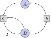
Example 1. Consider the CRN N = (S, R, F) with S = {A, B}, R = {a, b}, F(a) = (A+B,2B) andF(b) = (B, A). This CRN is taken from [16] (see also [1]). This example is the running example of this section.
We now define a natural digraph for a CRNN, called the reaction graph of N. The name is from [11], and the concept is originally defined in [8].
Definition 2. Let N = (S, R, F)be a CRN. The reaction graphofN, denoted by RN, is the labeled digraph(V, R, F)with V ={in(r)|r∈R} ∪ {out(r)|r∈ R}.
Note that in the reaction graph each reactant and product vector becomes a sin-gle vertex. The vertices of the reaction graph are calledcomplexes. The reaction graph of the CRNN of our running example (Example1) is depicted in Fig.3.
A+B a 2B B b A
Fig. 3.The reaction graph of the CRN of Example1.
Aconfiguration cof N is a vectorc∈NS. Letr∈R. We say thatr canfire
Note thatc′ is a configuration as well. Moreover, we writec→c′ ifc→rc′ for
some r∈R. For τ ∈R∗ (as usual,R∗ is Kleene star onR) we writec→τ c′ if
c →τ1 c
1· · · →τn c′ where τ =τ1· · ·τn and τi ∈R for alli ∈ {1, . . . , n}. The reflexive and transitive closure of the relation→ is denoted by→∗. Ifc →∗ c′,
then we say thatc′isreachablefromc. We say that a configurationcisrecurrent
if for allc′ withc→∗c′ we havec′→∗c. Note that ifcis recurrent andc→∗c′,
thenc′ is recurrent.
Example 2. Consider again the running example. We have, e.g., 2A+B →aabb 2A+B. However, 2A+B is not recurrent as 2A+B →b 3Aand in configuration 3Ano reaction can fire. In fact, the recurrent configurations of N are precisely those that do not contain anyB. Indeed, assumecis recurrent. Then we can fire b until we obtain a configuration c′ that does not contain any B. No reaction
can fire forc′ and soc=c′ sincec is recurrent.
The definition of a CRN is equivalent to that of a Petri net [15]. In a Petri Net, species are called places p, reactions are called transitions, and configurations are calledmarkings. A Petri net is often depicted as a graph with two types of vertices, one type for the places and one for the transitions. The Petri net-style depiction of the running example is given in Fig.4. The round vertices are the places and the rectangular vertices are the transitions. We use in this paper several standard Petri net notions, which are recalled in the next subsection.
A
B
a b
2
Fig. 4.The Petri net-style depiction of the running example.
2.3 P/T-Invariants
The notions of this subsection are all taken from Petri net theory [15]. We first recall the notion of an incidence matrix of a CRN, which is not to be confused with the notion of an incidence matrix of a digraph (as recalled above). In fact, we will compare in the next subsection the incidence matrix of a CRN with the incidence matrix of its reaction graph.
Example 3. Consider again the CRNN of the running example. Then
IN =
a b A −1 1 B 1 −1
.
Note that ifc →τ c′, then c′ =c+INΦ(τ), where Φ(τ) denotes again the
Parikh image ofτ.
Av ∈NS is called a P-invariant ofN ifvTIN = 0 (here 0 denotes a zero vector of suitable dimension indexed by R). Similarly, v ∈ NR is called a
T-invariant of N ifINv = 0, i.e.,v ∈ker(IN).1 A P-invariant or T-invariant are also sometimes called P-semiflow and T-semiflow, respectively, in the literature. Observe that ifc→τ c′, thenΦ(τ) is a T-invariant if and only ifc′=c. A CRN
N is calledconservative if there is a P-invariantv such that supp(v) =S. Also, N is calledconsistent if there is a T-invariantvsuch that supp(v) =R.
A CRNN is said to bestructurally bounded when for every configurationc, there is a kc∈Nsuch that for each configuration c′ withc→∗c′ we have that
each entry of c′ is at mostkc. Note that for a structurally-bounded CRN, the
number of different configurations reachable from a given configuration is finite, and so for each configurationc, there is a recurrent configuration reachable from c. In this way, one often informally views the recurrent configurations as the possible states of the CRN in “the long term”.
The following result is well known.
Proposition 1 ([12]). LetN be a CRN. IfN is conservative, thenN is struc-turally bounded.
Example 4. The CRNNof the running example is both conservative and consis-tent. Indeed, anyv∈NSwithv(A) =v(B)≥1 is a P-invariant with supp(v) =S and anyw∈NRwithv(a) =v(b)≥1 is T-invariant with supp(v) =R.
2.4 Deficiency
The notions that we recall in this subsection are originally from chemical reaction theory (and are less studied within Petri net theory).
LetN = (S, R, F) be a CRN and letV ={in(r)|r∈R} ∪ {out(r)|r∈R}. We denote byYN theS×V matrix with for alls∈S andv∈V, entryYN(s, v) is equal tov(s).
The next lemma relates the incidence matrix IN of a CRN N with the incidence matrix of the reaction graphRN ofN.
Lemma 1 (Sect. 6 of [9]). Let N = (S, R, F)be a CRN. ThenIN =YNRN.
1 The P and T in P/T-invariant are short for Place and Transition (from Petri net
In the above equality,RN denotes the incidence matrixRN and not the graph. As a corollary to Lemma1, we have the following.
Corollary 1 ([11]). Let N= (S, R, F)be a CRN. Thenker(RN)⊆ker(IN).
The vectors v of ker(RN)∩NR, which are T-invariants by Corollary 1, are calledclosed T-invariants [3]. Recall that the vectorsvof ker(RN)∩NRdescribe the cycles of RN, and so for each closed T-invariant v of N, supp(v) does not contain any bridge ofRN. Since each of the entries of a T-invariant is nonnega-tive, the linear space ker(IN) does not necessarily have a basis consisting of only T-invariants, see Example5 below.
Thedeficiency δ(N) of a CRNN is r(RN)−r(IN). By Corollary1, δ(N) is non-negative. Thus, one may view δ(N) as a measure of the difference in dimensions between ker(RN) and ker(IN). The former is determined only by the structure of the reaction graph (ignoring the identity of the vertices), while the latter also incorporates the relations that rely on the identities of the vertices of the reaction graph.
Recall from Subsect.2.1 that r(RN) = |V(RN)| −c(RN). Hence, we have δ(N) = |V(RN)| −c(RN)−r(IN) [8,10]. Note that if δ(N) = 0, then every T-invariant ofN is closed and ker(RN) = ker(IN).
A+B a 2B A b B
Fig. 5.The reaction graph of a CRN discussed in Example5.
Example 5. In the running example, ker(RN) only contains the zero vector, while ker(IN) contains all scalar multiples of the vectorwwithw(a) =w(b) = 1. Thus ker(IN) has a basis consisting of only T-invariants. Moreover,δ(N) = 1. Alternatively, the reaction graphRN has 4 vertices and 2 connected components andr(IN) = 1. Thus,δ(N) = 4−2−1 = 1.
If we consider the CRNN′ of Fig.5, then ker(RN
′) also only contains the zero vector, while ker(IN′) contains all scalar multiples of the vector w with w(a) =−w(b) = 1. Again, δ(N′) = 1, however the only T-invariant of ker(IN
′) is the zero vector.
3
Dominance and Non-closed T-Invariants
Note that there is a natural partial order for the set of SCCs of a graph: for SCCsX andY, we haveX Y if there is a path from a vertex ofY to a vertex ofX. We now consider a different partial order, denoted by≤d, for the SCCs of a reaction graph of a CRN.
Lemma 2. Let N = (S, R, F) be a structurally-bounded CRN. Then the ≤d
relation between SCCs ofRN is a partial order.
For SCCsX andY we writeX <dY ifX≤dY andX =Y. We say thatX
dominates Y whenX <d Y. For a setS of SCCs, we let min≤d(S)⊆ S be the
set of elements ofS that are minimal with respect to the≤drelation among all the elements ofS.
Let us define for a SCC X of RN, out(X) = {r ∈ E(RN) | in(r) ∈ V(X),out(r)∈/ V(X)}. We call X terminal if out(X) = ∅. We call a reaction r (complexx, resp.)terminal ifr∈E(X) (x∈V(X), resp.) for some terminal SCCX ofRN.
We will consider the minimal setX of non-terminal SCCs that dominates all other non-terminal SCCs. In other words, if we letN be the set of non-terminal SCCs, thenX = min≤d(N).
LetB be the set of bridges ofRN. Theexit set of a setS of non-terminal SCCs, is a setZ ⊆B with both|Z|=|S| and|Z∩out(X)|= 1 for all X ∈ S. In other words,Z contains exactly one bridge of out(X) for each X∈ S.
Assuming the existence of a non-terminal reaction that can fire for some recurrent configurationc, the main result of this paper ensures the existence of certain sequencesτ withc′→τ c′ for some configurationc′reachable fromc. For
each exit set Z, there exists such a τ that avoids all bridges outsideZ and, at the same time, uses the bridges ofZ whenever possible. As a consequence, each of the sequencesτ corresponds to a T-invariantv=Φ(τ) that have zero entries for the bridges outsideZ and nonzero entries for some of the bridges insideZ. We will show that for various CRNs this necessary condition allows one to show that only terminal reactions can fire for all its recurrent configurations.
The proof idea is the following. Let us start with a recurrent configurationc. While traversing the configuration space by applying reactions starting fromc, we need never choose a bridge of RN going out of a SCCX that is dominated by someY (i.e.,Y <dX). Indeed, ifx∈V(X) andy∈V(Y) withy < x, then we may walk insideX toxandy < ximplies that any reactionrwith in(r) =y can fire for x. In this way we also avoid taking a reaction r′ with in(r′) =x.
Moreover, walking out ofY can be done by taking any of the bridges. We choose the one from the exit set Z. Now, eventually, our path insideRN will lead to a terminal vertex. However, since c is recurrent, we can go back toc. If a non-terminal reaction can fire forc, then this means that we can iterate this process (walking along bridges, etc.). Structural boundedness finally ensures that the configuration space is finite and so, we must eventually repeat a configuration that closes the “circuit”.
We are now ready to formulate the main result of this paper.
Theorem 1. Let N = (S, R, F) be a structurally-bounded CRN, and let X = min≤d(N), where N is the set of non-terminal SCCs ofRN. LetB be the set of bridges ofRN. Let Lbe the set of all non-terminal reactionsrof RN such that there is a non-terminal reactionr′ of RN within(r′)<in(r).
1. τ contains no reactions from(B\Z)∪L,
2. τ=π1σ1· · ·πnσn where eachπi is a path inRN from a non-terminal vertex
to a terminal vertex and eachσi is a sequence of terminal reactions, and 3. c′ →τc′ for some recurrent configuration c′ reachable fromc.
A a E C b D E+D d A+C
Fig. 6.The reaction graph of the CRN of Example6.
We illustrate Theorem1through a couple of examples.
Example 6. Consider the CRNN of Fig.6. It is easy to verify thatc=A+Cis a recurrent configuration. Moreover, there is a non-terminal reactionrthat can fire for this configuration (take r=aor r=b). Note that there is only one exit set Z for X, which is Z =B ={a, b, d}. By Theorem 1, there is aτ ∈R∗ such
that (1)τ contains no reactions from (B\Z)∪L, (2) τ is a sequence of paths, each going to a terminal vertex, and (3)c′ →τc′for some recurrent configuration
c′ reachable fromc. Indeed, we can choose, e.g.,τ =abdandc′=A+C.
A+C a E+C E+D b A+D
Fig. 7.The reaction graph of the CRN of Example7.
We now give another example.
Example 7. Consider the CRNN of Fig.7. It is easy to verify thatc=A+C+D is a recurrent configuration. Moreover, there is a non-terminal reaction r that can fire for this configuration (taker=a). We have thatZ =B={a, b}is the unique exit setZ forX. We notice thatτ=ab andc′ =A+C+D satisfy the
conditions of Theorem 1. Indeed, we have τ = τ1σ1τ2σ2 with τ1 = a, σ1 = ǫ (the empty string),τ2=b, andσ2=ǫ. Note that ifN contained the additional reactionA+D→dE+D, thenτ =abandc′=A+C+D would again satisfy
the conditions of Theorem 1, where τ=τ1σ1 withτ1=aandσ1=b.
Considering the non-closed T-invariantv=Φ(τ) withτ from Theorem1, we have the following corollary to Theorem1. Note that Condition2of Theorem1 implies that supp(v) contains a bridge, and thereforev(z)= 0 for somez∈Z.
Corollary 2. LetN,X,B, andLbe as in Theorem 1.
Assume there is an exit set Z of X such that there is no non-closed T-invariant v with (1) v(x) = 0for allx∈(B\Z)∪L and (2)v(z)= 0for some
z∈Z.
We remark that, in view of Theorem 1, Corollary 2 can be strengthened by replacing the condition v(z) = 0 for some z ∈ Z with the stronger (but more involved) condition that says that the (occurrences of the) non-terminal reactions ofv form a set of paths where each path ends in a terminal vertex.
Note that since closed T-invariantsvcannot contain bridges, we may without loss of generality remove the condition thatv is “non-closed” in Corollary2.
We use Corollary2 to determine whether no non-terminal reaction can fire for any recurrent configuration of a CRN. While non-closed T-invariants have a central role in Corollary 2, curiously, this notion from [3] has been given only modest attention in both the Petri net theory and the CRN theory.
For a given exit set Z of X, one can verify using linear programming in polynomial time whether or not there is a non-closed T-invariant v with the properties of Corollary2. While in general there may be an exponential number of exit sets (exponential in the number of reactions) to check, in many cases the number of exit sets is severely constraint and in these cases the sufficient condition of Corollary2is computationally efficient.
A
Fig. 8.The reaction graph of the CRN of Example8.
We now give some examples to illustrate Corollary2.
together with the two non-closed T-invariants v1=Φ(gf ce) and v2=Φ(hf ce). We remark thatA+H+D→gf ceA+H+DandC+H+D→hf ceC+H+D. Thus δ(N) = 2. Note thatB ={e, f, g, h} is the set of bridges of RN. LetX be the set of non-terminal SCCs of RN that are minimal with respect to ≤d. We notice that Z = {e, f} is the only exit set of X. Also L = {g, h}. Now, the non-closed T-invariants v1 andv2 are witnesses that there is no non-closed T-invariantvwith both (1)v(g) =v(h) = 0 (note that (B\Z)∪L={g, h}) and (2) eitherv(e) orv(f) nonzero. By Corollary2, for every recurrent configuration no non-terminal reaction can fire. Since every reaction is non-terminal, for every recurrent configuration no reaction can fire.
A+B a 2B B+C b A+C
Fig. 9.The reaction graph of the CRN of Example9.
The next example shows that the converse of Theorem1 does not hold.
Example 9. Consider the CRNN of Fig.9. We show that no reaction can fire for any recurrent configuration ofN. Letcbe a recurrent configuration. Ifcdoes not contain any C, then we can fire reactiona until we obtain a configuration c′ for which no more reactions can fire. Sincec is recurrent, c =c′ and we are
done. Ifccontains at least oneC, then we can apply reactionbuntil we obtain a configurationc′′ with onlyA’s andC’s. Hence no reaction can fire forc′′. Since
c is recurrent, we havec=c′′and we are done.
However, for c =A+B+C we have c →τ c with τ =ab. We notice that Z ={a, b}is the only exit set ofX and (B\Z)∪L=∅. Thusτ trivially contains no reactions from (B\Z)∪Landτ=π1π2with pathsπ1=aandπ2=binRN from non-terminal vertices to terminal vertices. This shows that the converse of Theorem 1does not hold.
We remark that if we remove speciesCfrom reactionb(in this way obtaining the running example of Sect.2), then Corollary2 (and Theorem1) would have been applicable to show that no (non-terminal) reaction can fire for any recurrent configuration ofN.
4
Using Rates
This paper is inspired by the main technical result of [1] (cf. Theorem 3.3 of the supplementary material of [1]). In this section we recall its result. First we recall a particular matrix. Let R≥0 (R>0, resp.) be the set of nonnegative (positive, resp.) real numbers.
Definition 4. Let N = (S, R, F)be a CRN. LetV =V(RN)and letκ∈RR >0.
We denote byKN,κ the S×V matrix where for eachx∈V the column ofKN,κ
belonging toxis equal to
The value κ(r) in Theorem 2 may be interpreted as the “rate” of reaction r. Note that the definition of KN,κ is closely related to the definition of IN (Definition3).
We are now ready to formulate the main technical result of [1].
Theorem 2 ([1]). LetN= (S, R, F)be a conservative CRN andV =V(RN). Let L be the set of non-terminal vertices v of RN such that there is a non-terminal vertexv′ ofRN withv′< v. Assume thatL=∅.
If some non-terminal reaction can fire for some recurrent configuration c, then for allκ∈RR
>0, there is aw∈ker(KN,κ)∩R≥V0 withsupp(w)∩L=∅ and
there is a non-terminal vertexxwith x∈supp(w).
Theorem2 is proved in [1] using both intricate probabilistic arguments and methods from mass action kinetics. In [1], the theorem is unnecessarily stated in a probabilistic fashion using the notion of “positive recurrent configuration” for stochastically modeled CRNs: it can be stated in a deterministic way (see Theorem2 above) by realizing that the configuration space is finite for a given initial configuration in a structurally-bounded CRN. This deterministic formu-lation and the discrete model (in contrast to mass action) triggered the search of this paper for a combinatorial explanation of this result. We invite the reader to compare the proof techniques used to prove Theorem2in [1] and Theorem1 in this paper.
2B b A+B a 2A
Fig. 10.The reaction graph of the CRN of Example10.
Note that ifL=∅, then Theorem2is silent. We now show an example with L=∅ where Corollary2can be applied.
Example 10. Consider the CRN N of Fig.10. Note thatN is conservative with w(A) =w(B) = 1 as a witness. The only T-invariants v of N are those where v(a) =v(b). LetZ ={a} be an exit set ofX. Then there is no non-closed T-invariantvwithv(b) = 0 andv(a)= 0. By Corollary2, no non-terminal reaction can fire for any recurrent configurationcofN. Since all reactions ofN are non-terminal, no reaction can fire for any recurrent configuration c of N. Indeed, one observes that the recurrent configurations of N are those configurations containing either onlyA’s or onlyB’s, for whichaandbcannot fire.
A+D
Fig. 11.The reaction graph of the CRN of Example11.
Example 11. Consider the CRN N of Fig.11. Note thatN is conservative with w(X) = 1 for all species X as a witness. Note that A+D < 2A+D and so none of the non-closed T-invariants ofNcontains a bridge and so by Corollary2, no non-terminal reaction can fire for any recurrent configuration of N.
Conversely, despite trying numerous examples, we could not find an example where Theorem2predicts that no non-terminal reaction can fire for any recurrent configuration, but where Theorem 1is silent.
5
Discussion
Based on structural properties of CRNs, the main result of this paper (cf. Theorem 1) provides a sufficient condition to analyze the long-term behavior of CRNs. While its proof is using basic combinatorial arguments, the result is powerful enough to apply to a large class of CRNs. Also, the sufficient condition is computationally-efficient to verify for many CRNs. Another such sufficient condition is shown in [1], cf. Theorem 2. We have shown examples of CRNs where Theorem 1is applicable while Theorem2is silent.
T-invariant, which is crucial in the sufficient condition of Corollary2. This illus-trates that both research areas can significantly profit from each other.
An open problem is resolving whether Theorem 2 is indeed a special case of Theorem 1. Another open problem is to somehow strengthen Theorem 1 in a natural way to make it applicable for CRNs such as the one presented in Example9.
A further research direction is to incorporate probabilities. One may asso-ciate a probability to each T-invariant by multiplying the probabilities of the corresponding reactions. An open problem is to find a probabilistic version of Theorem 1to make predictions about long-term behavior of probabilistic com-putational models of CRNs, such as the models of [6,7,17].
Acknowledgements. We thank David Anderson for kindly explaining his work dur-ing the Banff International Research Station (BIRS) workshop on CRNs (14w5167). Also, we thank the organizers of this workshop during which this research was initiated. We are indebted to Matthew Johnston for carefully reading an earlier version of this paper and for providing useful comments. And in particular for finding a counterexam-ple to a conjecture in an earlier version of this paper. We finally thank the five referees for their useful comments. R.B. is a postdoctoral fellow of the Research Foundation – Flanders (FWO).
References
1. Anderson, D.F., Enciso, G.A., Johnston, M.D.: Stochastic analysis of biochemi-cal reaction networks with absolute concentration robustness. J. R. Soc. Interface 11(93), 20130943 (2014)
2. Aris, R.: Prolegomena to the rational analysis of systems of chemical reactions. Arch. Ration. Mech. Anal.19(2), 81–99 (1965)
3. Boucherie, R.J., Sereno, M.: On closed support T-invariants and the traffic equa-tions. J. Appl. Probab.35(2), 473–481 (1998)
4. Brijder, R.: Dominance and deficiency for Petri nets and chemical reaction net-works. arXiv preprint,arXiv:1503.04005(2015)
5. Chen, H.-L., Doty, D., Soloveichik, D.: Deterministic function computation with chemical reaction networks. In: Stefanovic, D., Turberfield, A. (eds.) DNA 2012. LNCS, vol. 7433, pp. 25–42. Springer, Heidelberg (2012)
6. Cook, M., Soloveichik, D., Winfree, E., Bruck, J.: Programmability of chemical reaction networks. In: Condon, A., Harel, D., Kok, J.N., Salomaa, A., Winfree, E. (eds.) Algorithmic Bioprocesses. Natural Computing Series, pp. 543–584. Springer, Berlin Heidelberg (2009)
7. Cummings, R., Doty, D., Soloveichik, D.: Probability 1 computation with chemical reaction networks. In: Murata, S., Kobayashi, S. (eds.) DNA 2014. LNCS, vol. 8727, pp. 37–52. Springer, Heidelberg (2014)
8. Feinberg, M.: Complex balancing in general kinetic systems. Arch. Ration. Mech. Anal.49(3), 187–194 (1972)
10. Horn, F.: Necessary and sufficient conditions for complex balancing in chemical kinetics. Arch. Ration. Mech. Anal.49(3), 172–186 (1972)
11. Mairesse, J., Nguyen, H.: Deficiency zero Petri nets and product form. Fundam. Inf.105(3), 237–261 (2010)
12. Memmi, G., Roucairol, G.: Linear algebra in net theory. In: Brauer, W. (ed.) Net Theory and Applications. Lecture Notes in Computer Science, vol. 84, pp. 213–223. Springer, Heidelberg (1975)
13. Oxley, J.: Matroid theory, 2nd edn. Oxford University Press, Oxford (2011) 14. Paulev´e, L., Craciun, G., Koeppl, H.: Dynamical properties of discrete reaction
networks. J. Math. Biol.69(1), 55–72 (2014)
15. Reisig, W., Rozenberg, G. (eds.): APN 1998. LNCS, vol. 1491. Springer, Heidelberg (1998)
16. Shinar, G., Feinberg, M.: Structural sources of robustness in biochemical reaction networks. Science327(5971), 1389–1391 (2010)
Networks with Specified Behaviours
Neil Dalchau, Niall Murphy(B), Rasmus Petersen, and Boyan Yordanov
Microsoft Research, Cambridge, CB1 2FB, UK {ndalchau,a-nimurp,a-rapete,yordanov}@microsoft.com
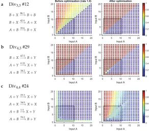
Abstract. We consider how to generate chemical reaction networks (CRNs) from functional specifications. We propose a two-stage approach that combines synthesis by satisfiability modulo theories and Markov chain Monte Carlo based optimisation. First, we identify candidate CRNs that have the possibility to produce correct computations for a given finite set of inputs. We then optimise the reaction rates of each CRN using a combination of stochastic search techniques applied to the chem-ical master equation, simultaneously improving theprobabilityof correct behaviour and ruling out spurious solutions. In addition, we use tech-niques from continuous time Markov chain theory to study the expected termination time for each CRN. We illustrate our approach by identify-ing CRNs for majority decision-makidentify-ing and division computation, which includes the identification of both known and unknown networks.
Keywords: Chemical reaction networks
·
Program synthesis·
Para-meter optimisation·
Chemical master equation·
Satisfiability modulo theories·
Markov chain Monte Carlo1
Introduction
A central goal of molecular programming is to be able to implement arbitrary dynamical behaviours. Chemical reaction networks (CRNs) are a popular for-malism for describing biochemical systems, such as protein interaction networks, gene regulatory networks, synthetic logic circuits and molecular programs built from DNA. Extensive theoretical understanding exists about the behaviour of a multitude of CRNs, and the behaviour of some networks has been exhaustively explored [1]. Besides describing chemical systems, CRNs provide a common lan-guage for expressing problems studied in computer science theory (e.g. Petri nets, network protocols) as well as control theory and engineering. Methods exist to convert CRNs into equivalent physical implementations, based on DNA strand displacement [2,3] the DNA toolbox system [4] and genelets [5]. Therefore, we sought to develop a methodology for proposing candidate CRNs that exhibit a pre-specified behaviour.
The computational power of CRNs has been extensively studied [6]. It is known that error-free (stably computing [7]) CRNs compute exactly the class of
c
Springer International Publishing Switzerland 2015
semi-linear functions [8,9]. However, if the stability restriction is relaxed and we allow the CRN to sometimes compute the wrong answer then it is possible to implement a register machine, that is, CRNs with error can compute functions beyond the semi-linear class (indeed they are equivalent in power to Turing machines) [6,10].
Although there are procedures to generate CRNs for semi-linear func-tions [8,10], primitive recursive functions [6], or even from arbitrary Turing machines [6], the proposal of practical (i.e. experimentally implementable) CRNs that compute a given function has thus far mostly been a manual effort. In this work, we attempt to automate the proposal of CRNs, by formally specifying a behaviour and automatically identifying CRNs that satisfy the desired behaviour with high probability. First, we formalise the problem of identifying CRNs that have the capacity to produce correct, finite computations for a given finite set of inputs. This corresponds to a synthesis problem, as opposed to verification, where the goal is to determine the correctness of a given CRN [11]. We express CRN synthesis as a satisfiability modulo theories (SMT) problem, which can be addressed using solvers such as Z3 [12]. This allows us to generate a number of candidate CRNs or to prove that no such CRN of a given size (in terms of numbers of reactions, species and computation lengths) exists. However, while the existence of correct computations is guaranteed for each generated CRN, the probability of these computations might be low.
To determine whether correct computations can occur with high probabil-ity, we next optimise the reaction rates of each generated CRN. To solve the optimisation problem, we combine stochastic search strategies based on Markov chain Monte Carlo (MCMC) with numerical integration of the chemical master equation (CME). This part of the problem was recently addressed in [13,14], though applied only to a single input.
In this paper, we specifically focus on uniform CRNs, those that have a fixed number of species and reactions for all input sizes.We also restrict our atten-tion to bimolecular CRNs, where there are precisely 2 reactants and 2 products in every reaction. Bimolecular CRNs are equivalent to Population Protocols (PPs) [7] and also guarantee that mass is conserved in the system. We applied our two-step approach first to majority decision-making, in which the network seeks to identify which of two inputs is in an initial majority. Majority networks are well-studied in the literature, and there are many known CRNs that give approximate solutions [15–17]. We then applied our approach to division, a non-linear function which has been relatively less studied. We show a range of CRNs for majority and division identified automatically using our method, some of which have been identified and characterised previously, though some of which are entirely novel. This illustrates the potential for automatically determining CRNs with a specified behaviour.
2
Preliminaries
A chemical reaction network (CRN) is a tupleC= (Λ,R), where Λ ={s0, . . . , sn}
A reaction is a tupler= (rr,pr, kr) whererrandprare the reactant and product stoichiometryvectors (rr
s ∈ N0 andprs ∈ N0 denote the stoichiometry of each
speciess ∈ Λ), kr ∈ R
≥0 denotes the rate ofrandkdenotes the vector of all
reaction rates. Given a reactionr = (rr,pr, kr), the set of reactants ofris{s ∈ Λ | rr
s >0}and the set of products ofris{s ∈ Λ | prs >0}. In this paper, we focus on the class ofbimolecularCRNs, where
s∈Λrrs= 2 and
s∈Λprs= 2, for all reactionsr∈ R.
The dynamical behaviour of bimolecular CRNs can be understood as fol-lows. The set of all possible system states isX =N|Λ|0 , where a statex∈N|Λ|0 represents the number of molecules of each species. We denote the number of molecules of speciess∈Λ at statexbyxs. Given a reactionr∈ Rwhererr The time at which reaction r would fire, once the system enters state x∈ X, is stochastic and follows an exponential distribution with a rate determined by the reaction’s propensitykr
x. Assuming that reactionris the first one to fire, the state of the system is updated asx′
s=xs−rrs+prs for alls∈Λ, wherexand
x′ are the current and next states.
An abstraction of CRNs that preserves reachability but does not consider reaction rates or time is given by thetransition systemTC = (X, T), where the
transition relationT is defined as
∀x, x′∈X . T(x, x′)↔
r∈R
s∈Λ
(xs≥rrs∧x′s=xs−rrs+prs). (1)
In other words, the choice between reactions from R is non-deterministic but enough molecules of each reactant must be present in statexfor the reaction to fire. The transition between states xandx′ happens when any reactionr∈ R
fires and the number of molecules is updated accordingly. A path x0, x1, . . . of T satisfiesT(xi, xi+1) fori= 0,1, . . .and, given an initial statex0we call state
xf reachable from x0 if there exists a pathx0, . . . , xf.
Given a CRNC, letX0⊆X denote a finite set of initial states andXr⊆X denote the set of states reachable fromX0. Assuming thatXris finite,C can be represented as a continuous time Markov chain (CTMC) that preserves infor-mation about the transition probabilities and rates that determine the sto-chastic behaviour of the system and the expected execution times. We define a CTMC to be a tuple M = (Xr, π0,Q), where Xr is a finite set of states,
π0:Xr→Ris the initial distribution of molecule copy numbers of all species, and Q :Xr×Xr → Ris a matrix of transition propensities. While the set of initial states is not represented explicitly, it is captured through the initial dis-tribution, i.e.X0 ={x∈Xr|π0(x)>0}. A CTMCMC is constructed from a
CRNCby first determining the set of reachable states, and then evaluating the propensities of each reaction. The (i, j)th entry ofQ,q
ij, represents a transition from state xi to state xj. Accordingly, qii is the remaining probability mass,
1 We assume that the reaction volume is 1 to allow for later volume scaling e.g.kr x/v
equal to −
i=jqij. The transient probability vector πt evolves according to dπt
dt =πtQ, which is known as the chemical master equation (CME).
Following [13,14], a parametric CTMC (pCTMC) is a CTMC where the reaction rates are parameterised by k, as above. Denote by P the parameter space,P :RP
≥0, such thatkis instantiated by a parameter pointp∈ P.
Accord-ingly, given a pCTMC M and parameter space P, an instantiated pCTMC
Mp= (X, π0,Qp) is an evaluation at pointp∈ P.
3
Problem Formulation
The main problem we consider in this paper, which we formalise in this section, is the identification of CRNs that satisfy given properties. Specifically, we are interested in finite reachability properties, which capture a range of interesting CRN behaviours.
Let C = (Λ,R) be a given CRN and TC = (X, T) and MC = (X
r, π0,Q)
denote its transition system abstraction and CTMC representation, as discussed in Sect.2. Letφ:X→Bdenote astate predicate, constructed using
φ: : =Eb
Eb : : =true|false|Ec| ¬Eb|Eb⊲Eb where ⊲∈ {∧,∨,⇒,⇔}
Ec : : =Ea⊲Ea where⊲∈ {<,≤,=, >,≥}
Ea : : =s∈Λ|c∈Z|Ea⊲Ea where⊲∈ {+,−,∗}.
For example, if φ:=s >5, thenφ(x) denotes that xs>5.
In this paper, we considerpath predicatesΦ = (φ0, φF), which are expressed using two state predicates that must be satisfied at the initial (φ0) and at some
final (φF) state of a path. LetK denote the number of steps we consider.
Definition 1. Given a finite path ρ : x0. . . xK of TC we say that ρ satisfies path predicate Φ = (φ0, φF), denoted as ρ Φ, if and only if φ0(x0)∧φF(xK) evaluates to true and no reactions are enabled in xK (i.e. xK is a terminal state).2
We define the probability of Φ, denotedPΦ, usingMC as follows. LetX0= {x∈X |φ0(x)} denote the set of states that satisfy the initial state predicate.
We initialise MC with a uniform sample from the states that satisfyφ
0, which
definesπ0 as
2 We consider terminating computations by enforcing that no reactions are enabled at
the state that satisfiesφF. Alternative strategies possible within our approach could
consider reaching a fix-point (i.e. the firing of any enabled reaction does not cause a transition to a different state), or reaching a cycle along whichφF is satisfied, to
π0(x) =
1
|X0| ifx∈X0 0 otherwise
Similarly, XF ={x∈X | φF(x)} denotes the set of states satisfying the final state predicate.
Definition 2. The probability ofΦis defined as
PΦ=
x∈XF πt(x),
wheretdenotes the maximal time we consider andπtis the probability vector at timet computed using the CME introduced in Sect.2. In other words, we define
PΦas the average probability of the states satisfying φF at timet.
Note that it is possible to optimise for both speed and accuracy by, for example, defining PΦto be the integration of the probability mass of all states satisfying
φF from time 0 to timet.
Problem 1. Given a finite set of path predicates{Φ0, . . . ,Φn}, find a bimolecular
CRNC such that
1. for each Φi, there exists a pathρi ofTC, such thatρiΦi and 2. the average probability
n i=0PΦi
n+1 defined usingMC is maximised.
4
Synthesis and Tuning of CRNs
We solve Problem1by addressing each of the two subproblems separately. First, we generate a number of CRNs that satisfy the specifications from Problem1.1 using a satisfiability modulo theories (SMT)-based approach (Sect.4.1). The CRNs identified at that point are capable of producing a path that satisfy each path predicate, which addresses Problem1.1 but they might also include incor-rect paths and the probability of corincor-rect computations might be low. Therefore, we tune the reaction rates of these CRNs in order to maximise the average probability (discussed in Sect.4.2), which addresses Problem1.2
4.1 SMT-Based Synthesis
Here, we present our approach to finding a bimolecular CRN C that satisfies a specification expressed as path predicates {Φ0, . . . ,Φn} (Problem1.1). We
address this problem by encoding TC symbolically for any possible
bimolecu-lar CRNC= (Λ,R) where|R|=M and|Λ|=N (i.e. the number of species and reactions is given), together with the specification{Φ0, . . . ,Φn}for some finite
we apply an incremental procedure to search for CRNs of increasing complexity (larger N andM) or to provide more complete results by increasing K.
Using Z3’s theory of linear integer arithmetic, we represent the stoichiom-etry of C as two symbolic matrices r ∈ N0M×N and p ∈ NM0 ×N (using integer constraints to prohibit negative integers). Given a reaction r ∈ R and species
s ∈ Λ, rr
s (prs) defined in Sect.2 is now encoded as a symbolic integer. We ensure that only bimolecular CRNs are considered by asserting the constraints
M−1
j=0 pi,j = 2. In addition, we introduce the
following constraints.
– We label a subset of the species ΛI ⊆ Λ as inputs and assert that
s∈ΛI
r∈Rrrs>0 to ensure all inputs are consumed by at least one reaction. – We label a subset of the species ΛO ⊆ Λ as outputs and assert that
reactions never have the same reactants and products and, therefore, all M
reactions are utilised. – Finally, we assert that
r∈R
s∈Λprs =rrs to ensure that the firing of each reaction updates the state of the system.
Following an approach inspired by bounded model checking (BMC) [18], we represent the finite path ρi = xi0, . . . xiK for each Φi by defining each state as a symbolic vector xi
j ∈ NN0 and “unrolling” the transition relation of TC (i.e.
asserting the constraint T(xi
j, xij+1) for each i = 0. . . n and j = 0. . . K−1).
s∈Λxs <rrs, i.e. no reactions are possible due to insufficient molecules of at least one reactant.
The parameter K specifies the maximal trajectory length that is consid-ered. The BMC approach is conservative, since computations that require more than K steps (reaction firings) to reach a state satisfying φF will not be iden-tified. Increasing K leads to a more complete search, and indeed the approach becomes complete for a sufficiently large K determined by the diameter of a system, but also increases the computational burden. To alleviate this, we follow an approach from [11] and considerstutter transitions (corresponding to multi-ple firings of the same reaction in a single step) by using the following modified transition relation definitionTst(as opposed to T from Eq.1)
species needed for the reaction to fire (xs ≥ n·(rrs−prs)). In many cases, stutter transitions dramatically decreases the required trajectory lengths (K), since multiple copies of the same species can react simultaneously. However, this is not restrictive, since for n = 1 the original definition of T is recovered. In addition to such stutter transitions,Tst allows self loops at terminal states, and therefore computations that require less thanKsteps to reach a state satisfying
φF can also be identified.
The encoding strategy described so far allows us to represent CRN synthesis as an SMT-problem and apply an SMT solver such as Z3 [12] to produce a CRN that satisfies the specification or prove that no such CRN exists for the choice ofM,N andK. More specifically, a solution CRNC is represented through the valuation ofrandp, which are extracted from themodelreturned by Z3.
In general, we are interested in enumerating many (or all possible) CRNs for the given class (defined byM, N andK), which ensures that no valid solu-tions are omitted at that stage. To do so, we apply an incremental SMT-based procedure, where at each step we assert an uniqueness constraint guaranteeing that no previously discovered CRNs are generated. Given a concrete, previously generated CRN C′ = (Λ,R′) and the new symbolic CRN C = (Λ,R) we are
searching for (both of which are defined using the same species Λ), we define the constraint DifferentFrom(C′) ¬ permutation of the same reactions3. We start by generating a solutionC′(if one
exists), asserting the constraintDifferentFrom(C′), and repeating this procedure
until the constraints become unsatisfiable, which corresponds to a proof that not additional CRNs exists for the givenN,M, and K.
4.2 Tuning CRNs with Parameter Optimisation
Here, we present our approach to optimising the reaction rates for CRNs
satisfy-ing{Φ0, . . . ,Φn}. This becomes a parameter synthesis problem over a pCTMC
set, analogous to parameter synthesis for a single pCTMC, as studied in [13,14]. In contrast to this work, we aggregate over the multiple input combinations, as specified in Problem1.2.
To obtain solutions for the probability at a specified timeπt, we used numer-ical integration of the CME. Specifnumer-ically, we used the Visual GEC software (http://research.microsoft.com/gec) to encode the CRNs and then integrate the CME for each combination of inputs.
To solve the maximisation problem, we used a Markov chain Monte Carlo (MCMC) method, as implemented in the Filzbach software (http://research. microsoft.com/filzbach). Filzbach uses a variation of the Metropolis-Hastings (MH) algorithm to perform Bayesian parameter inference. The MH algorithm is used to approximate the posterior probability of a parameter set from a hypoth-esised model taking on certain values, constrained by a likelihood function. The
3 At present, our uniqueness constraint does not consider other CRN isomorphisms
probability of each parameter value is then approximated by constructing a Markov chain of sampled parameter sets, such that a proposed parameter set is accepted with some probability, based on the ratio of the likelihood func-tion evaluated at current and proposal parameter sets. For more informafunc-tion on MCMC methods, see [19]. MCMC methods, such as simulated annealing, have also been shown to efficiently find solutions to combinatorial optimisation problems [20], taking a stochastic search approach similar to the MH algorithm. Stochastic search can provide benefits over gradient-based optimisers by main-taining a nonzero probability of making up-hill moves, protecting against getting stuck in poor local optima. To use Filzbach for providing solutions to optimi-sation CRN parameters, it is sufficient to encode the argument of Problem1.2 as a likelihood function. Subsequently, we generate MCMC chains with suit-ably many burn-in iterations and samples to obtain an approximate optimising parameter setk.
4.3 Calculating Expected Time
To evaluate the temporal performance of a CRN algorithm C, we make use of Markov chain theory to obtain the expected time until a terminal state is reached. This is an exact measure of the expected running time for a given pCTMC with inputs i ∈ I, as opposed to using the mean of many stochastic simulations [10].
LetA⊆Xr be the absorbing states of a pCTMCMCp = (X, π0,Qp) and let
τA be a vector of expected hitting times, corresponding to the expected time of transitioning from a state x ∈ Xr to A. Then τA can be evaluated as the solution to the equations (page 113 of [21])
τxA= 0 forx∈A
−
x′∈Xr
qx,x′τxA′ = 1 forx /∈A.
Numerical solutions can be obtained by forming a matrix W where the rows and columns ofQp corresponding to the terminal states (A) have been removed. Then, τA is the solution toW τA =1, where 1is the vector of 1’s. Numerical solutions can be obtained using Gaussian elimination.
Note that the time complexity analysis of CRNs typically assumes a volume
n equal to the maximum number of molecules in the system at any time [8] (equivalent to parallel time in PPs [10]). This volume can be included by dividing each propensity by nbefore calculating expected time (see Sect.2). In the case of bimolecular CRNs this is equivalent to multiplyingτA byn.
5
Case Studies
5.1 Approximate Majority
exactly computed by bimolecular CRNs (or population protocols) with less than 4 species [22]. For CRNs with 2 and 3 species there are known optimal (in terms of reaction firings) approximate algorithms [15,16].
We specify the majority problem using the path predicate (see Sect.2): ΦAM(a, b) := (φ0(a, b), φF(a, b)), where
sis. We applied the SMT approach to identify all CRNs with 2 to 4 reactions and 2 or 3 species that satisfy ΦAM for K ≤5 stutter steps (for N species and M
reactions, there areN2
(N2
−1)
M
total possible CRNs). We used a short optimisa-tion (20 burn-in, 20 samples) and sorted these soluoptimisa-tions by the value of PΦAM
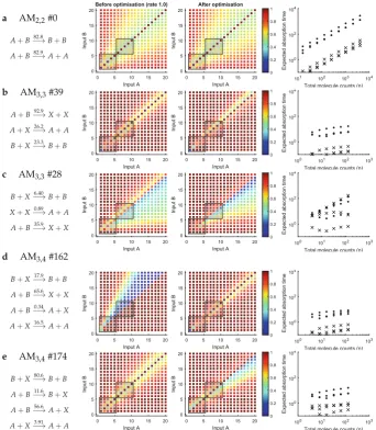
for each. We then applied a longer optimisation (700 burn-in, 700 samples) to the top 10 CRNs (Fig.1).
2 reactions 3 reactions 4 reactions
AM2,2
Before optimisation After short optimisation After long optimisation
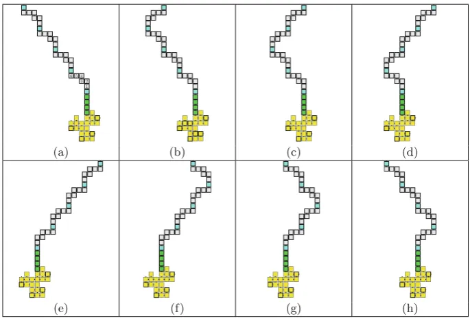
Fig. 1. Performance of approximate majority circuits.The SMT-based method was applied to the approximate majority specification for CRNs with 2, 3 and 4 reac-tions. For each category, the top 10 CRNs satisfying ΦAM are ordered by their average
probability after a short optimisation (20 burn-in, 20 samples; red bars). A longer optimisation (700 burn-in, 700 samples; green bars) was also performed. We also show the average probabilities before optimisation (all rates equal to 1.0; blue bars). The dashed line is the average probability of CRNAM3,4 #448 after the longer
Fig. 2.Response of Approximate Majority algorithms to varied inputs. For each input combination, specified as initial copies of species A and species B, the probability that both have the correct molecule count after 100 time units is reported. Results are shown for a variety of networks that performed well following optimisation (see Fig.1). The performance of each CRN is compared both before optimisation (all rates equal to 1.0; left panels) and after long optimisation (central panels). The grey boxes show the input ranges used for both generation and optimisation. The expected time until the CTMC reaches a terminal state is calculated for varying total molecule counts (n) (right panels). These times consider rates scaled as if occurring in a volume n
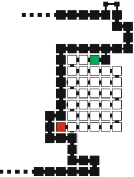
Using our approach, we found 1 CRN with 2 reactions and 2 species, the known direct competition (DC) network [23] (Fig. 2a). Out of 59,640 possible CRNs with 3 species and 3 reactions, the SMT solver found 39 CRNs where ΦAM was satisfied, 2 of which with probability over 0.696 after the short opti-misation (see Fig. 1). These two networks (AM3,3 #24 and AM3,3 #28) are
the dual of each other and behave asymmetrically but perform well owing to a compensatory asymmetric parameterisation (Fig.2c). One might expect that we should discover the known approximate majority circuit [15,17], (see Fig. 2b). However, this CRN does not satisfy the specification ΦAM since, for input (A= 1, B= 1, X= 0) the network terminates in the state (A= 0, B= 0, X = 2) and thus fails to make a decision. If we remove this single problematic input from the specification ΦAM, then this CRN is indeed discovered. We include it for comparison asAM3,3#39. Note that it scores a 0 on inputsA= 1, B= 1.
By increasing the number of reactions to 4, the SMT solver found 515 sat-isfying networks out of the 1,028,790 possible ones. The top 5 networks,AM3,4
#448, #328, #445, #333, and #257 have the same rules as the 3 reaction net-workAM3,3#39 but each has a different 4th reaction. The networkAM3,4#162
had a lower performance than AM3,3 #39 before optimisation and was almost
as good following optimisation. This network was also asymmetric, with a corre-sponding asymmetric parameterisation after optimisation (Fig.2d). The known 4 reaction networkAM3,4#174 [17] (Fig.2e) is also identified in 10th position.
Finally, we analysed the expected time until termination for each circuit, using the procedure in Sect.4.3 (right-hand panels of Fig. 2). Note that Defi-nition 2 does not reward circuits that reach a high probability before the final time tf = 100. However, in nearly all cases, the estimated hitting time of each system was improved by optimisation.
Computation Times. The computation times of our procedure depend on the size of the circuit (M andN), length of considered computations (K) and exact specification Φ (including the number of given path predicates). We illustrate the computation times required for the SMT-based synthesis part of our approach with the majority decision-making CRNs (Fig.3).
To determine how the CME calculation used in our method scales with mole-cular copy numbers, we first ran calculations of the CME for the established 3-reaction approximate majority CRN (system AM3,3 #39). The calculation
was initialised with 0.6n copies of A and 0.4n copies of B, and all rates were set to 1. As increasing the copy number decreases the simulation time inter-val over which there are transient dynamics, we integrated the CME over the time interval
0,100n
, wherenis the total copy number. We calculated transient probabilities at 500 output points, withn∈[10,1000]. This led to state-spaces of varying size, up to 106, with all calculations completing within 7200 s (2 h) (Fig.4). Smaller examples took only a few seconds.