If the observed value of the test-statistic , the the null hypothesis should be reject and accepted

The majority of hypothesis tests discussed so far have made inferences about population parameters, such as the mean and the proportion. These parametric tests have used the parametric statistics of samples that came from the population being tested. To formulate these tests, we made restrictive assumptions about the populations from which we drew our samples. For example, we assumed that our samples either were large or came from normally distributed populations. But populations are not always normal.

And even if a goodness-of-ft test indicates that a population is approximately normal. We cannot always be sure we’re right, because the test is not 100 percent reliable.

Fortunately, in recent times statisticians have develops useful

techniques that do not make restrictive assumption about the

shape of population distribution.

These are known as distribution – free or, more commonly,

nonparametric test.

Non parametric statistical procedures in preference to their parametric counterparts.

NON PARAMETRIC TESTS

SIGN TEST

WILCOXON SIGNED RANK TEST

MANN – WHITNEY TEST (WILCOXON RANK SUM TEST)

RUN TEST

KRUSKAL – WALLIS TEST

KOLMOGOROV – SMIRNOV TEST

The sign test is used to test hypotheses about the

median of a continuous distribution. The median

of a distribution is a value of the random variable X

such that the probability is 0,5 that an observed

value of X is less than or equal to the median, and

the probability is 0,5 that an observed value of X is

greater than or equal to the median. That is,

Since the normal distribution is symmetric, the

mean of a normal distribution equals the median.

Therefore, the sign test can be used to test

Let X denote a continuous random variable with

median and let

denote a random sample of

size n from the population of interest.

If denoted the hypothesized value of the

population median, then the usual forms of the

hypothesis to be tested can be stated as follows :

(right-tailed test)

(right-tailed

test) (left-tailed _test) (left-tailed

test) (two-tailed _test) (two-tailed

test)

Form the diferences :

Now if the null hypothesis is true,

any diference is equally likely to be positive

or negative. An appropriate test statistic is the

number of these diferences that are positive,

say . Therefore, to test the null hypothesis we are

really testing that the number of plus signs is a value

of a Binomial random variable that has the parameter

p = 0,5 .

A p-value for the observed number of plus signs

can be calculated directly from the Binomial

distribution. Thus, if the computed p-value.

To test the other one-sided hypothesis,

vs

is less than or equal

α

,

we

will reject .

The two-sided alternative may also be

tested. If the hypotheses are:

It is also possible to construct a table of critical

value for the sign test.

As before, let denote the number of the

diferences that are positive and let

denote the number of the diferences that are

negative.

Let , table of critical values

for the sign test that ensure that

If the alternative is ,

then reject if .

If the alternative is ,

then reject if .

Since the underlying population is assumed to

be continuous, there is a zero probability that we

will fnd a “tie”d , that is , a value of exactly

equal to .

When ties occur, they should be set aside and

the sign test applied to the remaining data.

When , the Binomial distribution is

well approximated by a normal distribution

when n is at least 10. Thus, since the mean

of the Binomial is and the variance is

, the distribution of is approximately

normal with mean 0,5n and variance 0,25n

whenever n is moderately large.

Therefore, in these cases the null hypothesis

can be tested using the statistic :

THE NORMAL

Critical Regions/Rejection Regions for α-level

tests

versus

are given in this table :

CRITICAL/REJECTION REGIONS FOR

The sign test makes use only of the plus and minus signs of the diferences between the observations and the median (the plus and minus signs of the diferences between the observations in the paired case).

Frank Wilcoxon devised a test procedure that uses both direction (sign) and magnitude.

This procedure, now called the Wilcoxon signed-rank test.

The Wilcoxon signed-rank test applies to the case of the symmetric continuous distributions.

Under these assumptions, the mean equals the median.

THE WILCOXON SIGNED-RANK

Description of the test :

We are interested in testing,

Assume that is a random sample from a

continuous and symmetric distribution with

mean/median : .

Compute the diferences , i 1, 2, … n

Rank the absolute diferences , and then give

the ranks the signs of their corresponding diferences.

Let be the sum of the positive ranks, and be

the absolute value of the sum of the negative ranks,

and let .

Critical values of , say .

1. If , then value of the statistic ,

reject

If the sample size is moderately large (n>20),

then it can be shown that or has

approximately a normal distribution with mean

and

variance

Therefore, a test of can be based

on the statistic

Test statistic :

Theorem : The probability distribution of

when is true, which is based on a random

sample of size n, satisfes :

Proof :

Let if , then

where

For a given , the discrepancy has a

50 : 50 chance

The Wilcoxon signed-rank test can be applied to paired

data.

Let ( ) , j 1,2, …n be a collection of paired

observations from two continuous distributions that difer

only with respect to their means. The distribution of the

diferences is continuous and symmetric.

The null hypothesis is : , which is equivalent

to

.To use the Wilcoxon signed-rank test, the diferences are

frst ranked in ascending order of their absolute values,

and then the ranks are given the signs of the diferences.

Let be the sum of the positive ranks and

be the absolute value of the sum of the negative

ranks, and .

If the observed value , then is rejected

and accepted.

Eleven students were randomly selected from a large statistics class, and their numerical grades on two

successive examinations were recorded.

Use the Wilcoxon signed rank test to determine

whether the second test was more difcult than the

EXAMPLE

Studen t

solution :

Jumlah ranks positif :

Ten newly married couples were randomly selected, and each husband and wife were independently asked the question of how many children they would like to have. The following information was obtained.

Using the sign test, is test reason to believe that wives want fewer children than husbands?

Assume a maximum size of type I error of 0,05

EXAMPLE

COUPLE 1 2 3 4 5 6 7 8 9 10

WIFE X

Tetapkan dulu H

0

dan H

1

:

H

0

: p 0,5

vs H

1

: p < 0,5

Ada tiga tanda +.

Di bawah H

0

, S ~ BIN (9 , 1/2)

P(S ≤ 3) 0,2539

Pada peringkat α 0,05 , karena 0,2539 > 0,05

maka H

jangan ditolak.

SOLUSI

Pasangan 1 2 3 4 6 7 8 9 10

-Suppose that we have two independent

continuous populations X

1

and X

2

with means µ

1

and µ

2.

Assume that the distributions of X

1

and X

2

have the same shape and spread, and difer only

(possibly) in their means.

The Wilcoxon rank-sum test can be used to test

the hypothesis

H

0

: µ

1

µ

2.

This procedure is sometimes called

the Mann-Whitney test or Mann-Whitney U Test.

Let and be two

independent random samples of sizes

from the continuous populations X

₁

and X

_2.

We wish

to test the hypotheses :

H

₀

: µ

₁

= µ

₂

versus H

₁

: µ

₁

≠ µ

₂

The test procedure is as follows. Arrange all

n

1

+ n

2

observations in ascending order of magnitude and

assign ranks to them. If two or more observations

are tied, then use the mean of the ranks that would

have been assigned if the observations difered.

Let

W

₁

be the sum of the ranks in the smaller sample

(1), and defne

W

₂

to be the sum of the ranks in the

other sample.

Then,

Now if the sample means do not difer, we will expect

the sum of the ranks to be nearly equal for both

samples after adjusting for the diference in sample

size. Consequently, if the sum of the ranks difer

H

₀

: µ

₁

= µ

₂

is rejected, if either of the

observed values

When both n

₁

and n

₂

are moderately large,

say, greater than 8, the distribution of W

₁

can

be well approximated by the normal

distribution with mean :

and variance :

Therefore, for n

₁

and n

₂

> 8, we could use :

as a statistic, and critical region is :





two-tailed test





upper-tail test

A large corporation is suspected of sex-discrimination in the salaries of its employees. From employees with similar responsibilities and work experience, 12 male and 12 female employees were randomly selected ; their annual salaries in thousands of dollars are as follows :

Is there reason to believe that there random samples come from populations with diferent distributions ? Use α 0,05

EXAMPLE

Femal

es 22,5 19,8 20,6 24,7 23,2 19,2 18,7 20,9 21,6 23,5 20,7 21,6

H

₀

: f

₁

(x) f

₂

(x)



APA ARTINYA??

random samples berasal dari

populasi dengan distribusi yang sama

H

₁

: f

₁

(x) ≠ f

₂

(x)

Gabungkan dan buat peringkat salaries :

SOLUSI

SE

X GAJI

PERINGKA T

F 18,7 1

F 19,2 2

F 19,8 3

M 20,5 4

F 20,7 6

F 20,9 7

M 21,2 8

M 21,6 10

F 21,6 10

M 21,9 12

M 22,3 13

M 22,4 14

F 22,5 15

F 23,2 16

M 23,4 17

F 23,5 18

M 23,6 19

M 23,9 20

M 24,0 21

M 24,1 22

M 24,5 23

F 24,7 24

Andaikan, kita pilih sampel dari female, maka

jumlah peringkatnya

R

₁

R

_F

117

Statistic

Grafk

α 0,05

Z

hit

1,91

maka terima H

0

-1,96 1,96

The Kolmogorov-Smirnov Test (K-S) test is conducted by the comparing the hypothesized and sample cumulative distribution function.

A cumulative distribution function is defned as :

and the sample cumulative distribution function, S(x), is defned as the proportion of sample values that are less than or equal to x.

The K-S test should be used instead of the to determine if a sample is from a specifed continuous distribution.

To illustrate how S(x) is computed, suppose we have the following 10 observations :

110, 89, 102, 80, 93, 121, 108, 97, 105, 103.

We begin by placing the values of x in ascending

order, as follows :

80, 89, 93, 97, 102, 103, 105, 108, 110,

121.

Because x 80 is the smallest of the 10

values, the proportion of values of x that are

less than or equal to 80 is : S(80) 0,1.

X S(x) = P(X ≤ _x)

80 0,1

89 0,2

93 0,3

97 0,4

102 0,5

103 0,6

105 0,7

The test statistic D is the maximum- absolute

diference between the two cdf’s over all

observed values.

The range on D is 0 ≤ D ≤ 1, and the formula

is :

where

x = each observed value

S(x) = observed cdf at x

Let X

(1)

, X

(2)

, …. , X

(n)

denote the ordered

observations of a random sample of size n,

and defne the sample cdf as :

is the proportion of the number of

sample values less than

The Kolmogorov – Smirnov statistic, is defned to

be :

A state vehicle inspection station has been

designed so that inspection time follows a

uniform distribution with limits of 10 and 15

minutes.

A sample of 10 duration times during low

and peak trafc conditions was taken. Use

the K-S test with α 0,05 to determine if the

sample is from this uniform distribution. The

time are :

11,3 10,4 9,8 12,6 14,8

13,0 14,3 13,3 11,5 13,6

1.

H

₀

: sampel berasal dari distribusi Uniform

(10,15)

versus

H

1

: sampel tidak berasal dari distribusi

Uniform (10,15)

2.

Fungsi distribusi kumulatif dari sampel : S

Waktu Pengamata

n x S(x) F(x)

9,8 0,10 0,00 0,10

10,4 0,20 0,08 0,12

11,3 0,30 0,26 0,04

11,5 0,40 0,30 0,10

12,6 0,50 0,52 0,02

13,0 0,60 0,60 0,00

13,3 0,70 0,66 0,04

13,6 0,80 0,72 0,08

14,3 0,90 0,86 0,04

14,8 1,00 0,96 0,04

, untuk x 10,4

Dalam tabel , n 10 , α 0,05



D

10,0.05

0,41

f(D)

α P(D ≥ D

0

)

D

0

D

Suppose we have the following ten observations

110, 89, 102, 80, 93, 121, 108, 97, 105,

103 ;

were drawn from a normal distribution, with

mean µ 100 and standard-deviation σ 10.

Our hypotheses for this test are

H

0

: Data were drawn from a normal distribution,

with µ 100 and σ 10.

versus

H

1

: Data were not drawn from a normal

distribution, with µ 100 and σ 10.

F(x) P(X ≤ x)

SOLUTION

x F(x)

80 89 93 97 102 103 105 108 110 121

P(X ≤ 80) P(Z ≤ -2) 0,0228 P(X ≤ 89) P(Z ≤ -1,1) 0,1357

P(X ≤ 93) P(Z ≤ -0,7) 0,2420 P(X ≤ 97) P(Z ≤ -0,3) 0,3821 P(X ≤ 102) P(Z ≤ 0,2) 0,5793 P(X ≤ 103) P(Z ≤ 0,3) 0,6179 P(X ≤ 105) P(Z ≤ 0,5) 0,6915 P(X ≤ 108) P(Z ≤ 0,8) 0,7881 P(X ≤ 110) P(Z ≤ 1,0) 0,8413

x F(x) S(x)

80 0,0228 0,1 0,0772

89 0,1357 0,2 0,0643

93 0,2420 0,3 0,0580

97 0,3821 0,4 0,0179

102 0,5793 0,5 0,0793 =

103 0,6179 0,6 0,0179

105 0,6915 0,7 0,0085

108 0,7881 0,8 0,0119

110 0,8413 0,9 0,0587

Jika α 0,05 , maka critical value, dengan

n 10 diperoleh di tabel 0,409.

Aturan keputusannya, tolak H

₀

jika D > 0,409

Karena

H

₀

jangan ditolak atau terima H

₀

.

In most applications where we want to test for

normality, the population mean and the

population variance are known.

In order to perform the K-S test, however, we

must assume that those parameters are known.

The Lilliefors test, which is quite similar to the K-S

test.

The major diference between two tests is that,

with the Lilliefors test, the sample mean and

the sample standard deviation s are used

instead of µ and σ to calculate F (x).

LILLIEFORS TEST

A manufacturer of automobile seats has a production

line that produces an average of 100 seats per day.

Because of new government regulations, a new safety

device has been installed, which the manufacturer

believes will reduce average daily output.

A random sample of 15 days’ output after the

installation of the safety device is shown:

93, 103, 95 , 101, 91, 105, 96, 94, 101, 88, 98,

94, 101, 92, 95

The daily production was assumed to be normally

distributed.

Use the Lilliefors test to examine that assumption,

with α 0,01

Seperti pada uji K-S, untuk menghitung S (x) urutkan,

sbb :

SOLUSI

x S(x)

88 1/15 0,067

91 2/15 0,133

92 3/15 0,200

93 4/15 0,267

94 6/15 0,400

95 8/15 0,533

96 9/15 0,600

98 10/15 0,667

101 13/15 0,867

103 14/15 0,933

Dari data di atas, diperoleh dan s

4,85.

Selanjutnya F(x) dihitung sbb :

X F(x)

88

Akhirnya, buat rangkuman sbb :

Tabel, nilai kritis dari uji Lilliefors : α 0,01 , n 15 D_tab 0,257

maka

x F(x) S(x)

88 0,0401 0,067 0,0269

91 0,1292 0,133 0,0038

92 0,1788 0,200 0,0212

93 0,2358 0,267 0,0312

94 0,3050 0,400 0,0950

95 0,3821 0,533 0,1509 D

96 0,4602 0,600 0,1398

98 0,6255 0,667 0,0415

101 0,8238 0,867 0,0432

103 0,9115 0,933 0,0215

Usually a sample that is taken from a population

should be random.

The

runs test

evaluates the null hypothesis

H

0

: the order of the sample data is random

The alternative hypothesis is simply the negation

of H

0.

There is no comparable parametric test to

evaluate this null hypothesis.

The order in which the data is collected must be

retained so that the runs may be developed.

TEST BASED ON RUNS

DEFINITIONS :

1.

A run is defned as a sequence of the same

symbols.

Two symbols are defned, and each sequence

must contain a symbol at least once.

2.

A run of length j is defned as a sequence of j

observations, all belonging to the same group,

that is preceded or followed by observations

belonging to a diferent group.

For illustration, the ordered sequence by the sex of

the employee is as follows :

F F F M F F F M M F F M M M F F M F M M M M M

F

The sequence begins with a run of length three, followed by a run of length one, followed by another run of length three, and so on.

The total number of runs in this sequence is 11.

Let R be the total number of runs observed in an ordered sequence of n1 + n2 observations, where n1 and

n2 are the respective sample sizes. The possible values

of R are 2, 3, 4, …. (n1 + n2 ).

The only question to ask prior to performing the test is, Is the sample size small or large?

We will use the guideline that a small sample has n1 and

n2 less than or equal to 15.

In the table, gives the lower rL and upper rU values of

If

n

1

or

n

2

exceeds 15, the sample is

considered large, in which case a normal

approximation to f(r) is used to test H

0

versus

H

f(r)

r

AR

The mean and variance of R are determined to

be

normal

The Kruskal – Wallis H test is the nonparametric

equivalent of the Analysis of Variance F test.

It test the null hypothesis that all k populations

possess the same probability distribution against the

alternative hypothesis that the distributions difer in

location – that is, one or more of the distributions are

shifted to the right or left of each other.

The advantage of the Kruskall – Wallis H test over the

F test is that we need make no assumptions about the

nature of sampled populations.

A completely randomized design specifes that we

select independent random samples of n

1

, n

2

, …. n

k

THE KRUSKAL - WALLIS H

TEST

To conduct the test, we frst rank all :

n n

₁

+ n

₂

+ n

₃

+ … +n

_k

observations and compute

the rank sums, R

₁

, R

₂

, …, R

_k

for the k samples.

The ranks of tied observations are averaged in the

same manner as for the WILCOXON rank sum test.

Then, if H

₀

is true, and if the sample sizes n

₁

, n

₂

, …,

n

_k

each equal 5 or more, then the test statistic is

defned by :

will have a sampling distribution that can be

approximated by a chi-square distribution with (k-1)

degrees of freedom.

Therefore, the rejection region for the

test is , where is the value

that located α in the upper tail of the

chi- square distribution.

H0 : The k population probability distributions are identical

H1 : At least two of the k population probability

distributions

difer in location Test statistic :

where,

ni Number of measurements in sample i

Ri Rank sum for sample i, where the rank of each

measurementis computed according to its relative magnitude in the totality of data for the k samples. H0 : The k population probability distributions are identical

H1 : At least two of the k population probability

distributions

difer in location Test statistic :

where,

ni Number of measurements in sample i

Ri Rank sum for sample i, where the rank of each

measurementis computed according to its relative magnitude in the totality of data for the k samples.

KRUSKAL – WALLIS H TEST

n Total sample size n

1

+ n

2

+ … +n

k

Rejection Region : with (k-1) dof

Assumptions :

1. The k samples are random and independent

2. There are 5 or more measurements in each

sample

3. The observations can be ranked

No assumptions have to be made about the shape

of the population probability distributions.

n Total sample size n

₁

+ n

₂

+ … +n

_k

Rejection Region : with (k-1) dof

Assumptions :

1. The k samples are random and independent

2. There are 5 or more measurements in each

sample

3. The observations can be ranked

Independent random samples of three diferent brands of magnetron tubes (the key components in microwave ovens) were subjected to stress testing, and the number of hours each operated without repair was recorded. Although these times do not represent typical life lengths, they do indicate how well the tubes can withstand extreme stress. The data are shown in table (below). Experience has shown that the distributions of life lengths for manufactured product are often non normal, thus violating the assumptions required for the proper use of an ANOVA F test.

Use the K-S H test to determine whether evidence exists to conclude that the brands of magnetron tubes tend to difer in length of life under stress. Test using α 0,05

BRAND

A B C

Lakukan ranking/peringkat dan jumlahkan peringkat dari 3 sample tersebut.

H0 : the population probability distributions of length of life under

stress are identical for the three brands of magnetron tubes.

versus

H : at least two of the population probability

Solusi

A peringkat B peringkat C peringkat

36 5 49 8 71 14 48 7 33 4 31 3 5 2 60 12 140 15 67 13 2 1 59 11 53 9 55 10 42 6

Test statistic :

H

₀

???

f(H)

H

COMPARISON OF POPULATION

PROPORTIONS

Given X₁~BIN(n₁, p₁) and X₂~BIN(n₂, p₂) Statistics :

Are defned to be the sample proportions.

Assume, that X₁ and X₂ are independent;

2 2 2

1 1 1 ; ˆ ˆ n X p n X

p  

)

ˆ

(

)

ˆ

(

)

ˆ

ˆ

(

p

₁

p

₂

E

p

₁

E

p

₂

E







2 1

p

p





)

ˆ

(

)

ˆ

(

)

ˆ

ˆ

(

p

₁

p

₂

Var

p

₁

Var

p

₂

Var







2 2 2

1 1

1

(

1

)

(

1

)

For sufciently large n₁ and n₂ the standardized statistic :

The (1-α)100% CI :

As p₁ and p₂ UNKNOWN, approximate (1-α)100% CI for (p₁-p₂) :

2 2 2 2 1 1 1 2 1

)

1

(

)

1

(

)

ˆ

ˆ

(

z

_

n

p

p

n

p

p

p

p











2 2 2 1 1 1 2 1 2 1 ) 1 ( ) 1 ( ) ( ) ˆ ˆ ( n p p n p p p p p p       2 2 2 1 1 1 2 2 1

)

ˆ

1

(

ˆ

)

ˆ

1

(

ˆ

)

ˆ

ˆ

(

n

p

p

n

p

p

z

p

In the testing situation,

H_o : p₁ p₂ p ( p unknown ) Versus

Test statistic :

1

H

2 1

p

p



p

₁



p

₂

2 1

p

p





z

Z

RR

:



RR

:

Z





z

_

2

:

Z

z

_

RR



test los   2 1 2 1 ) 1 ( ) 1 ( ˆ ˆ n p p n p p p p Z     

EXAMPLE

Members of the Department of statistics at Iowa State Union collected the following data on grades in an introductory business statistics course and an introductory engineering statistics course.

Course #Students #A grades B.Stat 571 82

E.Stat 156 25

H_o : p₁ p₂ Vs

H₁ : p₁≠p₂

; The proportion of A grades in two courses is equal.

1436 ,

0 571

82 ˆ_{1  }

p 0,1603

156 25 ˆ_{2  }

1472 , 0 156 571 25 82 ˆ _    p ) 156 1 571 1 )( 8528 , 0 ( 1472 , 0 1603 , 0 1436 , 0    Z 52 , 0   Z

The p-value is 2P(Z≤-0,52) 0,6030 If α 5% < p-value

H_o would not be rejected

An insurance company is thinking about ofering discount on its life insurance policies to non smokers. As part of its analysis, it randomly select 200 men who are 50 years old and asks them if they smoke at least one pack of cigarettes per day and if they have ever sufered from heart diseases. The results indicate that 20 out of 80 smokers and 15 out of 120 non smokers sufer from heart disease. Can we conclude at the 5% los that smokers have a higher incidence of heart disease than non smokers ? DATA

berumur 50th

perokok

menderita penyakit

berumur 50th

bukan perokok menderita penyakit

EXERCIS E

Jelas Data Qualitative vs

Test statistic :

z_tab

Sample proportion : ;

Pooled proportion estimate : Value of the test statistic:

) 1 1 ( ˆ ˆ ) ˆ ˆ ( 2 1 2 1 n n q p p p z    . 645 , 1 :z  z z_0,05 

RR _ 25 , 0 80 20 ˆ_{1  }

p 0,125

120 15 ˆ_{2  } p 175 , 0 200 35 120 80 15 20 ˆ _{ }    p hit cal

z

z



ˆ₁ ˆ₂

p -p (0,25-0,125)

z= =

1 1 1 1

0 : p_{1 } p_{2 }







_tab

cal

z

z

2

,

28

reject

H

_o

Test statistic, is normally distributed

We can calculate p-value

p-value

Reject H_o

%

13

,

1

0113

,

0

)

28

,

2

(

z







SOAL-SOAL

1. Diberikan pmf dari variabel random X sbb: x 0 1 2 3

p(x) 0 k k 3k2

Tentukan k sehingga memenuhi sifat dari pmf!

x

x

p

(

)



0



1 3 0 ) ( 2     



p x k k k

0 1 2 3 2    k k 1 , 3 1 0 ) 1 )( 1 3

( k _ k _{  } k _ k _{ }



p

(

x

)



1

Untuk

Dengan demikian tidak memenuhi. Selanjutnya untuk

dapat diperiksa ternyata pada kondisi ini memenuhi sifat pmf.

Jadi nilai

0

1

)

1

(

1













p

k

0

1

)

2

(







p

1





k

3

1



k

3

1



In a public opinion survey, 60 out of a sample of 100 high-income voters and 40 out of a sample of 75 low-income voters supported a decrease in sales tax.

(a) Can we conclude at the 5% los that the proportion of voters favoring a sales tax decrease difers between high and low-income voters?

(b) What is the p-value of this test?

(c) Estimate the diference in proportions, with 99% confdence!

:

(

)

₀

2

1



p



p

H

_o

0

)

(

:

_{1 2}

1

p



p



H

96

,

1

:

z



RR

) ˆ ˆ

( p _ p

Solution:

53 , 0 75 40 ˆ ; 6 , 0 100 60

ˆ_{1  } p_{2  } p 571 , 0 175 100 75 100 40 60 ˆ _{ }    p 429 , 0 ˆ 1

ˆ _{ } p _ q 93 , 0 ) 75 1 100 1 )( 429 , 0 ( 571 , 0 ) 53 , 0 60 , 0 (     cal z 0 -1,96 1,96

(a) Conclusion : don not reject H_o

(b) p-value 2P(z > 0,93) 2(0,1762) 0,3524. (c)

TEST on MEANS WHEN THE OBSERVATIONS ARE PAIRED

TESTING THE PAIRED DIFFERENCES

Let (X₁, Y₁), (X₂, Y₂) … (X_n, Y_m) be the n pairs, where (X_i, Y_i) denotes the systolic blood pressure of the i th subject before and after the drug.

It is assumed that the diferences D₁, D₂, …, D_n constitute independent normally distributed RV such that:

and

TEST STATISTIC:

 

Di i

E _ Var D_i _D2

o D

o

H :







vs H₁ :



_D 



_o

n S

D T

D

o



 

D

Rejection criteria for testing hypotheses on means when the observation are paired

Null hypothesis Value test statistic under Ho

Alternative hypothesis Rejection criteria

Reject H_o when or when

o D

o

H :_{ }

n s d t d o   

Reject H_o when

Reject H_o when

1 , 2 



t

_n

t

_

o D

H₁ :_{ }

1 , 2 1 



t

_n

t

_

1 , 1 



t

_n

t

_

1 , 



t

_n

t

_

o D

H₁ :_{ }

o D

Pair Male Female Diference (male-female)

1 $ 14.300 $13.800 $ 500

2 16.500 16.600 -100

3 15.400 14.800 600

4 13.500 13.500 0

5 18.500 17.600 900

6 12.800 13.000 -200

7 14.500 14.200 300

8 16.200 15.100 1.100

9 13.400 13.200 200

Solution :

)

0

(

0

:



_D





₁





₂



o

H

vs

)

0

(

0

:

_{1 2}

1



D











H

Test statistic :

d

x

n

s

o

x

t

_D D D D







;

RR : reject H_o if : t > t_α ; t_0.05,9 1,833

400









n

D

x

d

_D i

t_cal falls in RR

Reject H_o at the los 0,05

Starting salary for males exceeds the starting

Consider a classroom where the students are given a test before they are taught the subject matter covered by the test. The student’s score on this pre test are

recorded as the frst data set. Next, the subject matter is presented to the class. After the instruction is

completed, the students are retested on the same

material. The scores on the second test, the post test, compose the second data set. It is reasonable to

expect that a student that scored high on the pre test will also score high on the post test(and vice versa). Inherently, a strong dependency exists between the members of a pair of scores generated by each

individual.

Student Pre test Post test D

1 54 66 12

2 79 85 6

3 91 83 -8

4 75 88 13

5 68 93 25

6 43 40 -3

7 33 78 45

8 85 91 6

9 22 44 22

10 56 82 26

11 73 59 -14

12 63 81 18

13 29 64 35

14 75 83 8

EX : Use the T statistic for the hypotheses

versus , which σ 1 to compute :

a) β, if α 0.05 and n 16 b) α, if β 0.025 and n 16 c) n, if α 0.05 and β 0.025

Solution: vs

H_o : μ = 5

H_o : μ = 5 H₁ : μ = 6

H₁ : μ = 6

μ = μ_o = 6 μ = μ₁ > μ_o

Test

Statistic :





n

X

T



(



)

RR = { > c}

X

(a)

P

(

X



c





5

)



0

.

05

05

.

0

5

5

(

X





c





05

.

0

)

5

(

4

(

T



c





P

05

.

0

)

(

T



t

_



P

753

,

1

15





t

t

_ , berarti

753

,

1

)

5

(

4

c





c 5.438

)

6

(

)

(

ˆ

₁













P

terima

H

o

H

benar

P

X

c

)

248

.

2

(

)

6

(

4

(













P

T

c

P

T



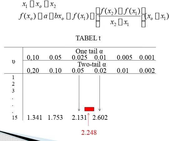
Tidak ada dalam tabel t JADI PAKAI INTERPOLASI

Umumnya, dipakai INTERPOLASI LINEAR

2 1

;

)

(

x

a

bx

x

x

x

2

1

x

x

x



_o



)

(

)

(

)

(

)

(

)

(

₁ 1 2 1 2

1

x

x

x

x

x

f

x

f

x

f

bx

a

x

f

_{o o}



_o

























TABEL t

One tail α

0,10 0.05 0.025 0.01 0.005 0.001 Two-tail α

0,20 0.10 0.05 0.02 0.01 0.002

)

(

)

(

)

(

)

(

)

(

₁ 1 2 1 2

1

x

x

x

x

x

f

x

f

x

f

x

f

_o



_o





















)

117

.

0

(

471

.

0

025

.

0

010

.

0

025

.

0

)

(



















o

x

f

021

.

0

)

(

x

_o



f

021

.

0

)

248

.

2

(









P

T



(b)

025

.

0

)

6

(













P

X

c

β = 0.025 ; n = 16 α = ?

025

.

0

)

6

(

4

(









P

T

c



025

.

042

.

0

)

868

.

1

(







P

T



Jadi : 4(c-6) -2,131 c 5,467

)

5

(

)

(











TABLE INTERPOLATION

Suppose that it is desired to evaluate a function f(x) at a point x_o , and that a table of values of f(x) is available for some, but not all, values of x. In particular, the table may not give the value f(x_o) but may give values for f(x₁) and f(x₂) where x₁< x_o< x₂ .

We can use the known values of f(x) for x x₁ , x₂ to approximate the value of f(x_o) .

This process is known as INTERPOLATION. Perhaps the most commonly used interpolation method is linear interpolation.

That is,

Solving the equations :

For a and b yields :

2 1

;

)

(

x

a

bx

x

x

x

f









2 2

1

1

)

;

(

)

(

x

a

bx

f

x

a

bx

f









1 2

1

2

)

(

)

(

x

x

x

f

x

f

b



























1 2 1 2 1

)

(

)

(

)

(

x

x

x

f

x

f

x

f

a

Hence :

)

(

)

(

)

(

)

(

)

(

₁ 1 2 1 2

1

x

x

x

x

x

f

x

f

x

f

bx

a

x

f

_{o o}



_o

























f(x₁)

f(x_o) f(x )

f(x)

EXERCISE

1. Let (X₁, X₂, …, X_n) be a random sample of a normal RV X with mean μ and variance 100. Let :

vs

As a decision test, we use the rule to accept H_o if , where

is the value of sample mean. a) fnd RR

b) fnd α and β for n 16.

2. Let (X₁, X₂, …, X_n) be a random sample of a Bernoulli R.V X with pmf:

where it is know that 0 < p ≤ . Let : vs

H_o : μ 50 H₁ : μ 55

53



x

x

2 1

H_o : p 1₂ H₁ : p p1( )

1

,

0

;

)

1

(

)

;

(

x

p



p



p

1

x



p

_X x x

(a) Find the power function γ(p) of the test. (b) Find α

(c) Find β : (i) if and (ii) p₁  p₂ 

4 1 10 1 Solutions : 2. a) b)

H_o : p = 1₂ vs H₁ : p = p1( ₂1 )

X~BER(p)

p

X

(

x

)



p

x

(

1



p

)

1x

;

x



0

,

1

)

(

)

(

p



P

reject

H

_o

p



2 1 0 ; ) 1 ( 20 ₂₀ 6 0              



_k pk p k p

k

)

2

1

(

)

2

1

(







P

reject

H

_o

p





1 1 1 20 ₂₀ 6 

c)



(

p

)



P

(

accept

H

_o

H

₁

is

true

)

2142 , 0 ) 4 3 ( ) 4 1 ( 20 1 ) 4 1

( 6 20

0             



k k

k k



)

(

1



P

reject

H

_o

p

₁



0024 , 0 ) 10 9 ( ) 10 1 ( 20 1 ) 10 1

( 6 20

0             



k k

k k

Let (X₁, X₂, …, X_n) be a random sample of a normal RV X with mean μ and variance 100. Let :

vs

As a decision test, we use the rule to accept H_o if . Find the value of c and sample size n such that α

0.025 and β 0.05.

H_o : μ = 50 H₁ : μ = 55

c

x



Solution :

}

:

)

,...,

,

{(

:

_{1 2}

1

x

x

x

x

c

R

_n



)

50

(

)

(













P

tolak

H

o

H

o

benar

P

X

c

025

.

0

)

10

50

(









n

c

Z

P



n= 52

975

.

0

)

(

Z



z

_



P

975

.

0

)

10

50

(







n

c

60

.

19

)

50

(

96

.

1

)

10

50

(







c



n



n

c

)

55

(

)

(

₁













P

terima

H

o

H

benar

P

X

c

05

.

0

)

10

55

(

05

.

0

)

10

55

(













n

c

n

c

P

45

.

16

)

55

(

645

.

1

10

)

55

(















n

c

n

29

.

3

)

50

(

92

.

3

)

55

(

55

29

.

3

50

92

.

3



















c

c

c

c

50

.

164

29

.

3

60

.

215

29

.

3

c







c



21

.

7

10

.

380

10

.

380

21

.

7

c





c



7184466

,

52

721

38010





c

718

.

52



c

60

.

19

)

50

(

c



n



Let (X₁, X₂, …, X_n) be a random sample of a normal RV X with mean μ and variance 36. Let :

vs

As a decision test, we use the rule to accept H_o if , where

is the value of sample mean.

a) Find the expression for the critical region/rejection region R₁ b) Find α and β for n = 16.

H_o : μ = 50 H₁ : μ = 55

53



x

x

Solution :

a) dimana

R

₁

:

{(

x

₁

,

x

₂

,...,

x

_n

)

:

x



53

}

)

2

(

)

50

53

(











P

X



P

Z





  n i i x n x 1 1

0228

.

0

9772

.

0

1

)

2

(

1













)

55

53

(

)

(

₁













P

terima

H

o

H

benar

P

X

)

333

.

1

(

)

333

.

1

(













P

Z



)

333

.

1

(

1









x₁ x_o x₂

1.330 1.333 1.340

0.9082 0.9099

1.330 1.340

)

330

.

1

333

.

1

(

330

.

1

340

.

1

9082

.

0

9099

.

0

9082

.

0

)

333

.

1

(











f

)

003

.

0

(

0100

.

0

0017

.

0

9082

.

0





90871

.

0

00051

.

0

9082

.

0

)

333

.

1

(







f

)

333

.

1

(

1









0913

.

0

90870

.

0

1



