By definition, two complex numbers are equal if and only if their real parts are equal and their imaginary parts are equal. (0, 1) is called the imaginary unit and is denoted by i,

608

C H A P T E R

1 3

Complex Numbers

and Functions. Complex

Differentiation

The transition from “real calculus” to “complex calculus” starts with a discussion of complex numbers and their geometric representation in the complex plane. We then progress to analytic functionsin Sec. 13.3. We desire functions to be analytic because these are the “useful functions” in the sense that they are differentiable in some domain and operations of complex analysis can be applied to them. The most important equations are therefore the Cauchy–Riemann equations in Sec. 13.4 because they allow a test of analyticity of such functions. Moreover, we show how the Cauchy–Riemann equations are related to the important Laplace equation.

The remaining sections of the chapter are devoted to elementary complex functions (exponential, trigonometric, hyperbolic, and logarithmic functions). These generalize the familiar real functions of calculus. Detailed knowledge of them is an absolute necessity in practical work, just as that of their real counterparts is in calculus.

Prerequisite: Elementary calculus.

References and Answers to Problems: App. 1 Part D, App. 2.

13.1

Complex Numbers and

Their Geometric Representation

The material in this section will most likely be familiar to the student and serve as a review.

Equations without real solutions, such as or were

observed early in history and led to the introduction of complex numbers.1

By definition, a complex numberzis an ordered pair (x, y) of real numbers xand y, written

z⫽_{(x, y).}

x2⫺_10x⫹₄₀⫽_0, x2⫽ ⫺₁

1

xis called the real partand ythe imaginary partof z, written

By definition, two complex numbers are equalif and only if their real parts are equal and their imaginary parts are equal.

(0, 1) is called the imaginary unitand is denoted by i, (1)

Addition, Multiplication. Notation

Additionof two complex numbers and is defined by (2)

Multiplicationis defined by (3)

These two definitions imply that

and

as for real numbers Hence the complex numbers “extend” the real numbers. We can thus write

because by (1), and the definition of multiplication, we have

Together we have, by addition,

In practice, complex numbers are written

(4)

or e.g., (instead of i4).

Electrical engineers often write jinstead of ibecause they need ifor the current. If then and is called pure imaginary. Also, (1) and (3) give

(5)

because, by the definition of multiplication, i2⫽_ii⫽_{(0, 1)(0, 1)}⫽₍⫺_{1, 0)}⫽ ⫺_1. i2⫽ ⫺₁

z⫽iy x⫽_0,

17⫹₄i z⫽x⫹yi,

z⫽x⫹iy zⴝ₍x,y)

(x, y)⫽_{(x, 0)}⫹_{(0, y)}⫽_x⫹_iy.

iy⫽_{(0, 1)y}⫽_{(0, 1)(y, 0)}⫽₍₀

#

_y⫺₁

#

_{0, 0}

#

₀⫹₁

#

_y)⫽_{(0, y).} (x, 0)⫽_{x. Similarly, (0, y)}⫽_iy

x1, x2.

(x1, 0)(x2, 0)⫽(x1x2, 0) (x1, 0)⫹(x2, 0)⫽(x1⫹x2, 0)

z1z2⫽(x1, y1)(x2, y2)⫽(x1x2⫺y1y2, x1y2⫹x2y1).

z1⫹z2⫽(x1, y1)⫹(x2, y2)⫽(x1⫹x2, y1⫹y2).

z2⫽(x2, y2)

z1⫽(x1, y1)

z

⫽

_x

⫹

_iy

i⫽_{(0, 1).} x⫽_{Re z, y}⫽_{Im z.}

For additionthe standard notation (4) gives [see (2)]

For multiplicationthe standard notation gives the following very simple recipe. Multiply each term by each other term and use when it occurs [see (3)]:

This agrees with (3). And it shows that is a more practical notation for complex numbers than (x, y).

If you know vectors, you see that (2) is vector addition, whereas the multiplication (3) has no counterpart in the usual vector algebra.

E X A M P L E 1 Real Part, Imaginary Part, Sum and Product of Complex Numbers

Let and . Then and

Subtraction, Division

Subtractionand divisionare defined as the inverse operations of addition and multipli-cation, respectively. Thus the difference is the complex number zfor which

Hence by (2),

(6)

The quotient is the complex number z for which If we equate the real and the imaginary parts on both sides of this equation, setting

we obtain The solution is

Complex numbers satisfy the same commutative, associative, and distributive laws as real numbers (see the problem set).

Complex Plane

So far we discussed the algebraic manipulation of complex numbers. Consider the geometric representation of complex numbers, which is of great practical importance. We choose two perpendicular coordinate axes, the horizontal x-axis, called the real axis, and the vertical y-axis, called the imaginary axis. On both axes we choose the same unit of length (Fig. 318). This is called a Cartesian coordinate system.

SEC. 13.1 Complex Numbers and Their Geometric Representation 611

y

x

1

1

P z = x + i y

(Imaginary axis)

(Real axis)

Fig. 318. The complex plane Fig. 319. The number 4 ⫺_3iin

the complex plane y

x

1

5

–1

–3 4 – 3i

We now plot a given complex number as the point Pwith coordinates x, y. The xy-plane in which the complex numbers are represented in this way is called the complex plane.2

Figure 319 shows an example.

Instead of saying “the point represented by zin the complex plane” we say briefly and simply “the point z in the complex plane.” This will cause no misunderstanding.

Addition and subtraction can now be visualized as illustrated in Figs. 320 and 321. z⫽_{(x, y)}⫽_x⫹_iy

y

x z₂

z₁

z₁+z₂

y

x

z₁–z₂ z₁ z₂

–z₂

Fig. 320. Addition of complex numbers Fig. 321. Subtraction of complex numbers

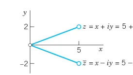
Fig. 322. Complex conjugate numbers y

x

5 2

–2

z= x + iy = 5 + 2i

z= x–iy = 5 – 2i

Complex Conjugate Numbers

The complex conjugate of a complex number is defined by

It is obtained geometrically by reflecting the point zin the real axis. Figure 322 shows this for z⫽₅⫹₂iand its conjugate z⫽₅⫺₂i.

z⫽x⫺iy.

z⫽x⫹iy z

The complex conjugate is important because it permits us to switch from complex to real. Indeed, by multiplication, (verify!). By addition and subtraction, We thus obtain for the real part x and the imaginary part y (notiy!) of the important formulas

(8)

If z is real, then by the definition of and conversely. Working with conjugates is easy, since we have

(9)

E X A M P L E 3 Illustration of (8) and (9)

Let and Then by (8),

Also, the multiplication formula in (9) is verified by

䊏

z1z2⫽(4⫺3i)(2⫺5i)⫽ ⫺7⫺26i.

(z1z2)⫽(4⫹3i)(2⫹5i)⫽(⫺7⫹26i)⫽ ⫺7⫺26i, Im z1⫽

1

2i[(4

⫹3i)⫺(4⫺3i)]⫽3i⫹3i

2i

⫽3.

z2⫽2⫹5i. z1⫽4⫹3i

(z1z2)⫽z1z2, a

z1

z2b

⫽z1 z2 .

(z1⫹z2)⫽z1⫹z2, (z1⫺z2)⫽z1⫺z2,

z, z⫽z

z⫽_x,

Re z⫽x⫽1_{2 (}z⫹z), Im z⫽y⫽ 1

2i(z⫺z). z⫽_x⫹_iy

z⫺_z⫽_2iy. z⫹_z⫽_2x,

zz⫽_x2⫹_y2

1. Powers of i. Show that and

2. Rotation. Multiplication by i is geometrically a counterclockwise rotation through p>2 (90°). Verify

1>i⫽ ⫺_{i, 1>i}2⫽ ⫺_{1, 1>i}3⫽_i,Á_.

i5⫽_i,Á

i2⫽ ⫺1, i3⫽ ⫺i, i4⫽1, this by graphing zand izand the angle of rotation for

3. Division. Verify the calculation in (7). Apply (7) to (26⫺18i)>(6⫺2i).

13.2

Polar Form of Complex Numbers.

Powers and Roots

We gain further insight into the arithmetic operations of complex numbers if, in addition to the xy-coordinates in the complex plane, we also employ the usual polar coordinates r, defined by

(1)

We see that then takes the so-called polar form

(2)

ris called the absolute valueor modulusof zand is denoted by Hence

(3)

Geometrically, is the distance of the point z from the origin (Fig. 323). Similarly, is the distance between and (Fig. 324).

is called the argumentof zand is denoted by arg z. Thus and (Fig. 323)

(4)

Geometrically, is the directed angle from the positive x-axis to OPin Fig. 323. Here, as in calculus, all angles are measured in radians and positive in the counterclockwise sense.

u

SEC. 13.2 Polar Form of Complex Numbers. Powers and Roots 613

4. Law for conjugates. Verify (9) for

5. Pure imaginary number. Show that is pure imaginary if and only if

6. Multiplication. If the product of two complex numbers is zero, show that at least one factor must be zero.

7. Laws of addition and multiplication. Derive the following laws for complex numbers from the cor-responding laws for real numbers.

(Commutative laws)

Let Showing the details of your work, find, in the form

8. 9.

For this angle is undefined. (Why?) For a given it is determined only up to integer multiples of since cosine and sine are periodic with period . But one often wants to specify a unique value of arg zof a given . For this reason one defines the principal valueArg z(with capital A!) of arg zby the double inequality

(5)

Then we have Arg for positive real which is practical, and Arg (not ) for negative real z, e.g., for The principal value (5) will be important in connection with roots, the complex logarithm (Sec. 13.7), and certain integrals. Obviously, for a given _z⫽_0,the other values of _{arg z are}arg z⫽_{Arg z} ⫾ _{2np (n}⫽ ⫾_1, ⫾_2,Á_).

(Fig. 325) has the polar form . Hence we obtain

and (the principal value).

Similarly, and

CAUTION! In using (4), we must pay attention to the quadrant in which zlies, since has period , so that the arguments of zand have the same tangent. Example: for and we u1⫽arg (1⫹i) u2⫽arg (⫺1⫺i) have tan u1⫽tan u2⫽1.

Fig. 323. Complex plane, polar form Fig. 324. Distance between two

of a complex number points in the complex plane

y

Inequalities such as make sense for realnumbers, but not in complex because there is no natural way of ordering complex numbers. However, inequalities between absolute values (which are real!), such as (meaning that is closer to the origin than ) are of great importance. The daily bread of the complex analyst is the triangle inequality

(6) (Fig. 326)

By induction we obtain from (6) the generalized triangle inequality (6*)

that is, the absolute value of a sum cannot exceed the sum of the absolute values of the terms. E X A M P L E 2 Triangle Inequality

If and then (sketch a figure!)

Multiplication and Division in Polar Form

This will give us a “geometrical” understanding of multiplication and division. Let

Multiplication. By (3) in Sec. 13.1 the product is at first

The addition rules for the sine and cosine [(6) in App. A3.1] now yield

(7)

Taking absolute values on both sides of (7), we see that the absolute value of a product equals theproductof the absolute values of the factors,

(8)

Taking arguments in (7) shows that the argument of a product equals the sum of the arguments of the factors,

(9) (up to multiples of ).

Division. We have Hence and by division by

(10) ` (z2⫽0).

z1

z2`

⫽ ƒz1ƒ

ƒz2ƒ

ƒz2ƒ

ƒz1ƒ ⫽ ƒ(z1>z2) z2ƒ ⫽ ƒz1>z2ƒ ƒz2ƒ

z1⫽(z1>z2)z2.

2p arg (z1z2)⫽arg z1⫹arg z2

ƒz1z2ƒ ⫽ ƒz1ƒ ƒz2ƒ.

z1z2⫽r1r2[cos(u1⫹u2)⫹i sin(u1⫹u2)].

z1z2⫽r1r2[(cos u1 cos u2⫺sin u1 sin u2)⫹i(sin u1 cos u2⫹cos u1 sin u2)].

z1⫽r1(cos u1⫹i sin u1) and z2⫽r2(cos u2⫹i sin u2).

䊏

ƒz1⫹z2ƒ⫽ƒ⫺1⫹4iƒ⫽117⫽4.123⬍12⫹113⫽5.020. z2⫽ ⫺2⫹3i,

z1⫽1⫹i

ƒz1⫹z2 ⫹Á⫹znƒ ⬉ ƒz1ƒ ⫹ ƒz2ƒ⫹Á⫹ƒznƒ;

SEC. 13.2 Polar Form of Complex Numbers. Powers and Roots 615

y

x z₂

z₁

z₁ + z₂

Similarly, and by subtraction of arg

(11) (up to multiples of ).

Combining (10) and (11) we also have the analog of (7),

(12)

To comprehend this formula, note that it is the polar form of a complex number of absolute value and argument But these are the absolute value and argument of as we can see from (10), (11), and the polar forms of and

E X A M P L E 3 Illustration of Formulas (8)–(11)

Let and Then . Hence (make a sketch)

and for the arguments we obtain

.

E X A M P L E 4 Integer Powers of z. De Moivre’s Formula

From (8) and (9) with we obtain by induction for

(13)

Similarly, (12) with and gives (13) for For formula (13) becomes

De Moivre’s formula3

(13*)

We can use this to express and in terms of powers of and . For instance, for we have on the left Taking the real and imaginary parts on both sides of with gives the familiar formulas

This shows that complexmethods often simplify the derivation of realformulas. Try .

Roots

If then to each value of wthere corresponds onevalue of z. We shall immediately see that, conversely, to a given there correspond precisely n distinct values of w. Each of these values is called an nth rootof z, and we write

z⫽₀ z⫽_wn _(n⫽_{1, 2,}Á_),

䊏

n⫽3 cos 2u⫽cos2u⫺sin2u, sin 2u⫽2 cos u sin u.

n⫽2

(13*) cos2_u⫹2

i cos u sin u⫺sin2_u.

n⫽2 sin u

cos u

sin nu

cos nu

(cos u⫹i sin u)n⫽cos nu⫹i sin nu.

ƒzƒ⫽r⫽1,

n⫽ ⫺1, ⫺2,Á.

z2⫽zn z1⫽1

zn⫽_rn (cos nu⫹_i sin nu).

n⫽0, 1, 2,Á

z1⫽z2⫽z

䊏

Arg (z1z2)⫽ ⫺ 3p

4

⫽Arg z1⫹Arg z2⫺2p, Arg a

z1 z2b

⫽p

4

⫽Arg z1⫺Arg z2

Arg z1⫽3p>4, Arg z2⫽p>2,

ƒz1z2ƒ⫽612⫽318⫽ ƒz1ƒ ƒz2ƒ, ƒz1>z2ƒ⫽212>3⫽ƒz1ƒ>ƒz2ƒ, z1z2⫽ ⫺6⫺6i, z1>z2⫽23⫹(

2 3)i z2⫽3i.

z1⫽ ⫺2⫹2i

z2.

z1

z1>z2, u1⫺u2.

r1>r2

z1

z2

⫽ r1

r2 [cos (u1

⫺_u2)⫹_{i sin (u1}⫺_u2)].

2p arg z_z1

2

⫽_arg z1⫺arg z2

z2 arg z1⫽arg [(z1>z2)z2]⫽arg (z1>z2)⫹arg z2

3

(14)

Hence this symbol is multivalued, namely, n-valued.The nvalues of can be obtained as follows. We write zand win polar form

Then the equation becomes, by De Moivre’s formula (with instead of ),

The absolute values on both sides must be equal; thus, so that where is positive real (an absolute value must be nonnegative!) and thus uniquely determined. Equating the arguments and and recalling that is determined only up to integer multiples of , we obtain

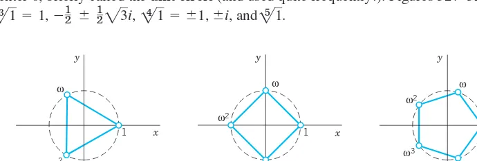
where kis an integer. For we get n distinctvalues of w. Further integers of kwould give values already obtained. For instance, gives , hence the wcorresponding to , etc. Consequently, for , has the ndistinct values

(15)

where These nvalues lie on a circle of radius with center at the origin and constitute the vertices of a regular polygon of nsides. The value of obtained by taking the principal value of arg zand in (15) is called the principal valueof

.

Taking in (15), we have and Arg Then (15) gives

(16)

These nvalues are called the nth roots of unity. They lie on the circle of radius 1 and center 0, briefly called the unit circle(and used quite frequently!). Figures 327–329 show 23

SEC. 13.2 Polar Form of Complex Numbers. Powers and Roots 617

If denotes the value corresponding to in (16), then the nvalues of can be written as

More generally, if is any nth root of an arbitrary complex number then the n values of in (15) are

(17)

because multiplying by corresponds to increasing the argument of by . Formula (17) motivates the introduction of roots of unity and shows their usefulness.

2kp>n

Represent in polar form and graph in the complex plane as in Fig. 325. Do these problems very carefully because polar forms will be needed frequently. Show the details.

1. 2.

3. 4.

5. 6.

7. 8.

9–14 PRINCIPAL ARGUMENT

Determine the principal value of the argument and graph it as in Fig. 325.

9. 10.

11. 12.

13. 14.

15–18 CONVERSION TO

Graph in the complex plane and represent in the form

15. 16.

17. 18.

ROOTS

19. CAS PROJECT. Roots of Unity and Their Graphs.

Write a program for calculating these roots and for graphing them as points on the unit circle. Apply the program to with Then extend the program to one for arbitrary roots, using an idea near the end of the text, and apply the program to examples of your choice.

20. TEAM PROJECT. Square Root. (a) Show that has the values

(18)

(b) Obtain from (18) the often more practical formula ( 1 9 )

where sign if sign if and all square roots of positive numbers are taken with positive sign. Hint:Use (10) in App. A3.1 with

(c) Find the square roots of and by both (18) and (19) and comment on the work involved.

(d) Do some further examples of your own and apply a method of checking your results.

21–27 ROOTS

Find and graph all roots in the complex plane.

21. 22. 23. 24.

25. 26. 兹81苶 27.

28–31 EQUATIONS

Solve and graph the solutions. Show details.

28. 29.

30. Using the solutions, factor into quadratic factors with realcoefficients.

13.3

Derivative. Analytic Function

Just as the study of calculus or real analysis required concepts such as domain, neighborhood, function, limit, continuity, derivative, etc., so does the study of complex analysis. Since the functions live in the complex plane, the concepts are slightly more difficult or different from those in real analysis. This section can be seen as a reference section where many of the concepts needed for the rest of Part D are introduced.

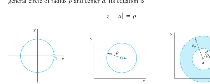
Circles and Disks. Half-Planes

The unit circle (Fig. 330) has already occurred in Sec. 13.2. Figure 331 shows a general circle of radius and center a. Its equation is

ƒz⫺_aƒ ⫽_r r

ƒzƒ ⫽₁

SEC. 13.3 Derivative. Analytic Function 619

32–35 INEQUALITIES AND EQUALITY

32. Triangle inequality. Verify (6) for

33. Triangle inequality.Prove (6).

z2⫽ ⫺2⫹4i

z1⫽3⫹i,

34. Re and Im.Prove

35. Parallelogram equality.Prove and explain the name

ƒz1⫹z2ƒ 2

⫹ ƒz1⫺z2ƒ 2

⫽2 (ƒz1ƒ 2

⫹ ƒz2ƒ 2

).

ƒRe zƒ⬉ ƒzƒ, ƒIm zƒ⬉ ƒzƒ.

y

x

1

y

x ρ

a

a y

x

1

ρ

2

ρ

Fig. 330. Unit circle Fig. 331. Circle in the Fig. 332. Annulus in the

complex plane complex plane

because it is the set of all zwhose distance from the center aequals Accordingly, its interior (“open circular disk”) is given by its interior plus the circle itself (“closed circular disk”) by and its exterior by As an example, sketch this for and to make sure that you understand these inequalities.

An open circular disk is also called a neighborhoodof aor, more precisely, a -neighborhoodof a. And ahas infinitely many of them, one for each value of

and ais a point of each of them, by definition!

In modern literature any setcontaining a -neighborhood of ais also called a neigh-borhoodof a.

Figure 332 shows an open annulus(circular ring) which we shall need later. This is the set of all zwhose distance from ais greater than but less than . Similarly, the closed annulus includes the two circles. Half-Planes. By the (open) upperhalf-planewe mean the set of all points

such that . Similarly, the condition defines the lower half-plane, the right half-plane, and x⬍₀the left half-plane.

x⬎₀ y⬍₀

y⬎₀

z⫽x⫹iy r1⬉ ƒz⫺aƒ ⬉r2

r2

r1

ƒz⫺aƒ

r1⬍ ƒz⫺aƒ ⬍r2, r

r (⬎_0), r

ƒz⫺aƒ ⬍_r

r⫽_2, a⫽₁⫹i

ƒz⫺aƒ ⬎_r.

ƒz⫺aƒ ⬉_r,

ƒz⫺aƒ ⬍_r,

r.

For Reference: Concepts on Sets

in the Complex Plane

To our discussion of special sets let us add some general concepts related to sets that we shall need throughout Chaps. 13–18; keep in mind that you can find them here.

By a point setin the complex plane we mean any sort of collection of finitely many or infinitely many points. Examples are the solutions of a quadratic equation, the points of a line, the points in the interior of a circle as well as the sets discussed just before.

A set Sis called open if every point of Shas a neighborhood consisting entirely of points that belong to S. For example, the points in the interior of a circle or a square form an open set, and so do the points of the right half-plane Re

A set Sis called connectedif any two of its points can be joined by a chain of finitely many straight-line segments all of whose points belong to S. An open and connected set is called a domain.Thus an open disk and an open annulus are domains. An open square with a diagonal removed is not a domain since this set is not connected. (Why?)

The complementof a set Sin the complex plane is the set of all points of the complex plane that do not belongto S. A set Sis called closedif its complement is open. For example, the points on and inside the unit circle form a closed set (“closed unit disk”) since its

complement is open.

A boundary pointof a set Sis a point every neighborhood of which contains both points that belong to Sand points that do not belong to S. For example, the boundary points of an annulus are the points on the two bounding circles. Clearly, if a set Sis open, then no boundary point belongs to S; if Sis closed, then every boundary point belongs to S. The set of all boundary points of a set Sis called the boundaryof S.

A regionis a set consisting of a domain plus, perhaps, some or all of its boundary points. WARNING!“Domain” is the modernterm for an open connected set. Nevertheless, some authors still call a domain a “region” and others make no distinction between the two terms.

Complex Function

Complex analysis is concerned with complex functions that are differentiable in some domain. Hence we should first say what we mean by a complex function and then define the concepts of limit and derivative in complex. This discussion will be similar to that in calculus. Nevertheless it needs great attention because it will show interesting basic differences between real and complex calculus.

Recall from calculus that a realfunction fdefined on a set Sof real numbers (usually an interval) is a rule that assigns to every xin Sa real number f(x), called the valueof fat x. Now in complex, Sis a set of complexnumbers. And a functionfdefined on Sis a rule that assigns to every zin Sa complex number w, called the valueof fat z. We write

Here z varies in Sand is called a complex variable. The set Sis called the domain of definitionof for, briefly, the domain of f. (In most cases Swill be open and connected, thus a domain as defined just before.)

Example: is a complex function defined for all z; that is, its domain Sis the whole complex plane.

The set of all values of a function fis called the rangeof f. w⫽_f(z)⫽_z2⫹_3z

w⫽_f(z). |zƒ ⬎₁

w is complex, and we write where uand v are the real and imaginary parts, respectively. Now wdepends on Hence ubecomes a real function of x and y, and so does v. We may thus write

This shows that a complexfunction f(z) is equivalent to a pairof realfunctions and , each depending on the two real variables xand y.

E X A M P L E 1 Function of a Complex Variable

Let Find uand vand calculate the value of fat .

Solution. and Also,

This shows that and Check this by using the expressions for uand v.

E X A M P L E 2 Function of a Complex Variable

Let Find uand vand the value of fat

Solution. gives and Also,

Check this as in Example 1.

Remarks on Notation and Terminology

1. Strictly speaking, f(z) denotes the value of f at z, but it is a convenient abuse of language to talk about the function f(z) (instead of the function f), thereby exhibiting the notation for the independent variable.

2. We assume all functions to be single-valued relations, as usual: to each zin Sthere corresponds but onevalue (but, of course, several zmay give the same value just as in calculus). Accordingly, we shall not use the term “multivalued function” (used in some books on complex analysis) for a multivalued relation, in which to a zthere corresponds more than one w.

Limit, Continuity

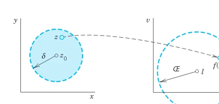
A function f(z) is said to have the limitlas zapproaches a point z0, written (1)

if f is defined in a neighborhood of (except perhaps at z0itself) and if the values of

fare “close” to lfor all z“close” to in precise terms, if for every positive real we can find a positive real such that for all in the disk (Fig. 333) we have (2)

geometrically, if for every in that -disk the value of flies in the disk (2). Formally, this definition is similar to that in calculus, but there is a big difference. Whereas in the real case, xcan approach an x0only along the real line, here, by definition,

d z⫽_z0

ƒf(z)⫺_lƒ ⬍P;

ƒz⫺_z0ƒ ⬍_d z⫽_z0

d

P

z0;

z0 lim z:z0 f(z)

⫽_l, w⫽_f(z),

w⫽_f(z)

䊏

f(12⫹4i)⫽2i( 1

2⫹4i)⫹6( 1

2⫺4i)⫽i⫺8⫹3⫺24i⫽ ⫺5⫺23i.

v(x, y)⫽2x⫺6y.

u(x, y)⫽6x⫺2y f(z)⫽2i(x⫹iy)⫹6(x⫺iy)

z⫽1₂⫹4i.

w⫽f(z)⫽2iz⫹6z.

䊏

v(1, 3)⫽15.

u(1, 3)⫽ ⫺5

f(1⫹3i)⫽(1⫹3i)2⫹3(1⫹3i)⫽1⫺9⫹6i⫹3⫹9i⫽ ⫺5⫹15i. v⫽2xy⫹3y.

u⫽Re f(z)⫽x2⫺y2⫹3x

z⫽1⫹3i w⫽f(z)⫽z2⫹3z.

v(x, y)

u(x, y) w⫽f(z)⫽u(x, y)⫹iv(x, y).

z⫽x⫹iy. w⫽u⫹iv,

Derivative

The derivativeof a complex function fat a point is written and is defined by

(4)

provided this limit exists. Then fis said to be differentiableat . If we write , we have and (4) takes the form

Now comes an important point. Remember that, by the definition of limit, f(z) is defined in a neighborhood of and zin ( ) may approach from any direction in the complex plane. Hence differentiability at z0means that, along whatever path zapproaches , the quotient in ( ) always approaches a certain value and all these values are equal. This is important and should be kept in mind.

E X A M P L E 3 Differentiability. Derivative

The function is differentiable for all zand has the derivative because

䊏

lim

¢z:0

z2⫹2z ¢z⫹(¢z)2⫺z2

¢z

⫽ lim

¢z:0(2z

⫹¢z)⫽2z.

fr(z)⫽ lim

¢z:0

(z⫹¢z)2⫺z2

¢z ⫽

fr(z)⫽2z f(z)⫽z2

4

r

z0

z0 4

r

z0

f

_r

(z0)⫽ lim z_:z0

f(z)⫺_f(z0) z⫺_z0 . (4

_r

)

z⫽z0⫹¢z

¢z⫽z⫺z0

z0

f

r

(z0)⫽ lim ¢z_:0

f(z0⫹¢z)⫺f(z0)

¢z

f

_r

(z0)

z0

y

x

v

u z

z₀ δ

f(z)

l

Œ

Fig. 333. Limit

zmay approach from any directionin the complex plane. This will be quite essential in what follows.

If a limit exists, it is unique. (See Team Project 24.)

A function f(z) is said to be continuousat if is defined and (3)

Note that by definition of a limit this implies that f(z) is defined in some neighborhood of .

f(z) is said to be continuous in a domainif it is continuous at each point of this domain. z0

lim z:z0 f(z)

⫽_f(z0). f(z0)

The differentiation rulesare the same as in real calculus,since their proofs are literally the same. Thus for any differentiable functions fand gand constant cwe have

as well as the chain rule and the power rule (ninteger).

Also, if f(z) is differentiable at z0, it is continuous at . (See Team Project 24.)

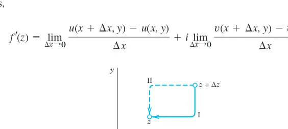
E X A M P L E 4 not Differentiable

It may come as a surprise that there are many complex functions that do not have a derivative at any point. For instance, is such a function. To see this, we write and obtain

(5)

If this is . If this is Thus (5) approaches along path I in Fig. 334 but along path II. Hence, by definition, the limit of (5) as ¢z:0does not exist at any z. _䊏

⫺1

⫹1

⫺1.

¢x⫽0,

⫹1

¢y⫽0,

f(z⫹¢z)⫺_f(z) ¢z

⫽(z

⫹¢z)⫺_z

¢z

⫽¢z

¢z

⫽¢x

⫺_i¢y

¢x⫹_i¢y.

¢z⫽¢x⫹_i¢y f(z)⫽_z⫽_x⫺_iy

z

z0 (zn)

_r

⫽nznⴚ1

(cf)

r

⫽cf

r

, (f⫹g)

r

⫽f

r

⫹g

r

, (fg)

r

⫽f

r

g⫹fg

r

, a_gfb

r

⫽ f

r

g ⫺fg

_r

g2

SEC. 13.3 Derivative. Analytic Function 623

Fig. 334. Paths in (5) y

x ΙΙ

Ι z + ∆z

z

Surprising as Example 4 may be, it merely illustrates that differentiability of a complex function is a rather severe requirement.

The idea of proof (approach of zfrom different directions) is basic and will be used again as the crucial argument in the next section.

Analytic Functions

Complex analysis is concerned with the theory and application of “analytic functions,” that is, functions that are differentiable in some domain, so that we can do “calculus in complex.” The definition is as follows.

D E F I N I T I O N Analyticity

A function is said to be analytic in a domain Dif f(z) is defined and differentiable at all points of D. The function f(z) is said to be analytic at a point in Dif f(z) is analytic in a neighborhood of .

Also, by an analytic functionwe mean a function that is analytic in somedomain.

Hence analyticity of f(z) at means that f(z) has a derivative at every point in some neighborhood of (including itself since, by definition, is a point of all its neighborhoods). This concept is motivated by the fact that it is of no practical interest if a function is differentiable merely at a single point but not throughout some neighborhood of . Team Project 24 gives an example.

A more modern term for analytic in Dis holomorphic in D. z0

z0

z0

z0

z0

z0

z0

E X A M P L E 5 Polynomials, Rational Functions

The nonnegative integer powers are analytic in the entire complex plane, and so are polynomials, that is, functions of the form

where are complex constants. The quotient of two polynomials and

is called a rational function. This fis analytic except at the points where here we assume that common factors of gand hhave been canceled.

Many further analytic functions will be considered in the next sections and chapters.

The concepts discussed in this section extend familiar concepts of calculus. Most important is the concept of an analytic function, the exclusive concern of complex analysis. Although many simple functions are not analytic, the large variety of remaining functions will yield a most beautiful branch of mathematics that is very useful in engineering and physics.

1–8 REGIONS OF PRACTICAL INTEREST

Determine and sketch or graph the sets in the complex plane given by

9. WRITING PROJECT. Sets in the Complex Plane.

Write a report by formulating the corresponding portions of the text in your own words and illustrating them with examples of your own.

COMPLEX FUNCTIONS AND THEIR DERIVATIVES

10–12 Function Values. Find Re f, and Im fand their values at the given point z.

10. 11. 12.

13. CAS PROJECT. Graphing Functions. Find and graph Re f, Im f, and as surfaces over the z-plane. Also

in the same figure, and the curves in another figure, where (a)

(b) , (c)

14–17 Continuity. Find out, and give reason, whether

f(z) is continuous at and for the function fis equal to:

14. 15.

16. 17.

18–23 Differentiation. Find the value of the derivative of

18. 19.

20. at any z. Explain the result.

21. at 0

22. at 2i 23.

24. TEAM PROJECT. Limit, Continuity, Derivative (a) Limit.Prove that (1) is equivalent to the pair of relations

(b) Limit. If exists, show that this limit is unique.

13.4

Cauchy–Riemann Equations.

Laplace’s Equation

As we saw in the last section, to do complex analysis (i.e., “calculus in the complex”) on any complex function, we require that function to be analytic on some domain that is differentiable in that domain.

The Cauchy–Riemann equations are the most important equations in this chapter and one of the pillars on which complex analysis rests. They provide a criterion (a test) for the analyticity of a complex function

Roughly, fis analytic in a domain Dif and only if the first partial derivatives of uand satisfy the two Cauchy–Riemann equations4

(1)

everywhere in D; here and (and similarly for v) are the usual notations for partial derivatives. The precise formulation of this statement is given in Theorems 1 and 2.

Example: is analytic for all z(see Example 3 in Sec. 13.3),

and and satisfy (1), namely, as well as

. More examples will follow.

T H E O R E M 1 Cauchy–Riemann Equations

Let be defined and continuous in some neighborhood of a point and differentiable at z itself. Then, at that point, the first-order partial derivatives of u andvexist and satisfy the Cauchy–Riemann equations(1). Hence, if is analytic in a domain D, those partial derivatives exist and satisfy (1) at all points of D.

f(z) z⫽x⫹iy

f(z)⫽u(x, y)⫹iv(x, y) ⫺₂y⫽ ⫺vx

uy⫽ ux⫽2x⫽vy

v⫽₂xy

u⫽x2⫺y2

f(z)⫽z2⫽x2⫺y2⫹₂ixy

uy⫽0u>0y ux⫽ 0u>0x

ux⫽vy, uy⫽ ⫺vx

v w⫽_f(z)⫽_{u(x, y)}⫹_{iv(x, y).}

SEC. 13.4 Cauchy–Riemann Equations. Laplace’s Equation 625

(d) Continuity.If is differentiable at show that

f(z) is continuous at

(e) Differentiability.Show that is not differentiable at any z. Can you find other such functions?

(f) Differentiability. Show that is dif-ferentiable only at z⫽0;hence it is nowhere analytic.

f(z)⫽ ƒzƒ2 f(z)⫽_{Re z}⫽_x

z0.

z0,

f(z) 25. WRITING PROJECT. Comparison with Calculus.

Summarize the second part of this section beginning with

Complex Function, and indicate what is conceptually analogous to calculus and what is not.

4

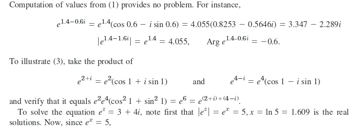
P R O O F By assumption, the derivative at zexists. It is given by

(2)

The idea of the proof is very simple. By the definition of a limit in complex (Sec. 13.3), we can let approach zero along any path in a neighborhood of z. Thus we may choose the two paths I and II in Fig. 335 and equate the results. By comparing the real parts we shall obtain the first Cauchy–Riemann equation and by comparing the imaginary parts the second. The technical details are as follows.

We write . Then and in terms of u

and vthe derivative in (2) becomes

(3) .

We first choose path I in Fig. 335. Thus we let first and then . After is zero, . Then (3) becomes, if we first write the two u-terms and then the two

v-terms,

f

r

(z)⫽ _lim

¢x:0

u(x⫹ ¢x, y)⫺u(x, y)

¢x

⫹i lim ¢x:0

v(x⫹¢x, y)⫺v(x, y)

¢x .

¢z⫽ ¢x

¢y

¢x:0

¢y:0 f

r

(z)⫽ _lim

¢z:0

[u(x⫹ ¢x, y⫹¢y)⫹iv(x⫹ ¢x, y⫹ ¢y)]⫺_[u(x, y)⫹iv(x, y)]

¢x⫹_i¢y

z⫹ ¢z⫽x⫹ ¢x⫹i(y⫹ ¢y),

¢z⫽ ¢x⫹i¢y

¢z

f

r

(z)⫽ _lim

¢z:0

f(z⫹ ¢z)⫺_f(z)

¢z .

f

_r

(z)

y

x ΙΙ

Ι z + ∆z

z

Fig. 335. Paths in (2)

Since exists, the two real limits on the right exist. By definition, they are the partial derivatives of uand vwith respect to x. Hence the derivative of f(z) can be written (4)

Similarly, if we choose path II in Fig. 335, we let first and then . After is zero, , so that from (3) we now obtain

Since exists, the limits on the right exist and give the partial derivatives of uand v

with respect to y; noting that we thus obtain (5)

The existence of the derivative thus implies the existence of the four partial derivatives in (4) and (5). By equating the real parts ux and vy in (4) and (5) we obtain the first

f

r

(z)

f

_r

(z)⫽ ⫺iu_y⫹v_y. 1>i⫽ ⫺_i,

f

r

(z)

f

_r

(z)⫽ _lim

¢y_:0

u(x, y⫹¢y)⫺u(x, y) i¢y

⫹i lim ¢y_:0

v(x, y⫹ ¢y)⫺_v(x, y)

i¢y .

¢z⫽i¢y

¢x

¢y:0

¢x:0 f

r

(z)⫽ux⫹ivx.

Cauchy–Riemann equation (1). Equating the imaginary parts gives the other. This proves the first statement of the theorem and implies the second because of the definition of analyticity.

Formulas (4) and (5) are also quite practical for calculating derivatives as we shall see. E X A M P L E 1 Cauchy–Riemann Equations

is analytic for all z. It follows that the Cauchy–Riemann equations must be satisfied (as we have verified above).

For we have and see that the second Cauchy–Riemann equation is satisfied, but the first is not: We conclude that is not analytic, confirming Example 4 of Sec. 13.3. Note the savings in calculation!

The Cauchy–Riemann equations are fundamental because they are not only necessary but also sufficient for a function to be analytic. More precisely, the following theorem holds.

T H E O R E M 2 Cauchy–Riemann Equations

If two real-valued continuous functions and of two real variables x and y have continuous first partial derivatives that satisfy the Cauchy–Riemann equations in some domain D, then the complex function is analytic in D.

The proof is more involved than that of Theorem 1 and we leave it optional (see App. 4). Theorems 1 and 2 are of great practical importance, since, by using the Cauchy–Riemann equations, we can now easily find out whether or not a given complex function is analytic. E X A M P L E 2 Cauchy–Riemann Equations. Exponential Function

Is analytic?

Solution. We have and by differentiation

We see that the Cauchy–Riemann equations are satisfied and conclude that f(z) is analytic for all z. (f(z) will be the complex analog of known from calculus.)

E X A M P L E 3 An Analytic Function of Constant Absolute Value Is Constant

The Cauchy–Riemann equations also help in deriving general properties of analytic functions.

For instance, show that if is analytic in a domain Dand in D, then in

D. (We shall make crucial use of this in Sec. 18.6 in the proof of Theorem 3.)

Solution. By assumption, By differentiation,

Now use in the first equation and in the second, to get

(6)

(a)

(b) uuy⫺vux⫽0.

uux⫺vuy⫽0, vy⫽ux

vx⫽ ⫺uy

uuy⫹vvy⫽0. uux⫹vvx⫽0,

ƒfƒ2_{⫽ ƒ}

u⫹_ivƒ2_⫽

u2⫹v2_⫽ k2.

f(z)⫽const ƒf(z)ƒ⫽k⫽const

f(z)

䊏

ex

uy⫽ ⫺_ex_{sin y,} vx⫽exsin y. ux⫽_ex_{cos y,} vy⫽excos y u⫽excos y, v⫽exsin y

f(z)⫽_{u(x, y)}⫹_iv(x, y)⫽_ex_{(cos y}⫹_{i sin y)}

f (z)⫽_{u(x, y)}⫹_{iv(x, y)}

v(x, y)

u(x, y)

䊏

f(z)⫽_z ux⫽₁⫽vy⫽ ⫺1.

uy⫽ ⫺vx⫽0,

u⫽_x, v⫽ ⫺_y f(z)⫽_z⫽x⫺iy

f(z)⫽_z2

f

r

(z),

䊏

To get rid of , multiply (6a) by uand (6b) by vand add. Similarly, to eliminate , multiply (6a) by and (6b) by uand add. This yields

If then hence If then Hence, by the

Cauchy–Riemann equations, also Together this implies and ; hence

We mention that, if we use the polar form and set , then the Cauchy–Riemann equationsare (Prob. 1)

(7)

Laplace’s Equation. Harmonic Functions

The great importance of complex analysis in engineering mathematics results mainly from the fact that both the real part and the imaginary part of an analytic function satisfy Laplace’s equation, the most important PDE of physics. It occurs in gravitation, electrostatics, fluid flow, heat conduction, and other applications (see Chaps. 12 and 18).

T H E O R E M 3 Laplace’s Equation

If is analytic in a domain D, then both u and v satisfy Laplace’s equation

(8)

( read “nabla squared”) and

(9) ,

in D and have continuous second partial derivatives in D.

P R O O F Differentiating with respect to xand with respect to y, we have

(10)

Now the derivative of an analytic function is itself analytic, as we shall prove later (in Sec. 14.4). This implies that uand vhave continuous partial derivatives of all orders; in particular, the mixed second derivatives are equal: By adding (10) we thus obtain (8). Similarly, (9) is obtained by differentiating with respect to y and

with respect to xand subtracting, using

Solutions of Laplace’s equation having continuoussecond-order partial derivatives are called harmonic functionsand their theory is called potential theory(see also Sec. 12.11). Hence the real and imaginary parts of an analytic function are harmonic functions.

䊏

u_xy⫽u_yx. u_y⫽ ⫺_vx

u_x⫽_vy

vyx⫽vxy.

u_xx⫽_vyx, u_yy⫽ ⫺_vxy.

u_y⫽ ⫺_vx u_x⫽_vy

ⵜ2_v⫽_vxx⫹_vyy⫽₀ ⵜ2

ⵜ2u⫽u_xx⫹u_yy⫽₀ f (z)⫽u(x, y)⫹iv(x, y)

vr⫽ ⫺

1 ruu

(r⬎_0). ur⫽

1 rvu,

iv(r, u)

f(z)⫽u(r, u) ⫹ z⫽r(cos u⫹i sin u)

䊏

f⫽const.

v⫽const

u⫽const

ux⫽vy⫽0.

ux⫽uy⫽0.

k2⫽u2⫹v2_⫽ 0,

f⫽0.

u⫽v⫽0;

k2⫽u2⫹v2_⫽ 0,

(u2⫹v2 )uy⫽_0. (u2⫹v2

)ux⫽_{0 ,}

⫺v

If two harmonic functions uand vsatisfy the Cauchy–Riemann equations in a domain D, they are the real and imaginary parts of an analytic function fin D. Then vis said to be a harmonic conjugate functionof uin D. (Of course, this has absolutely nothing to do with the use of “conjugate” for

E X A M P L E 4 How to Find a Harmonic Conjugate Function by the Cauchy–Riemann Equations

Verify that is harmonic in the whole complex plane and find a harmonic conjugate function vof u.

Solution. by direct calculation. Now and Hence because of the Cauchy– Riemann equations a conjugate vof umust satisfy

Integrating the first equation with respect to yand differentiating the result with respect to x, we obtain

.

A comparison with the second equation shows that This gives . Hence

(cany real constant) is the most general harmonic conjugate of the given u. The corresponding analytic function is

Example 4 illustrates that a conjugate of a given harmonic function is uniquely determined up to an arbitrary real additive constant.

The Cauchy–Riemann equations are the most important equations in this chapter. Their relation to Laplace’s equation opens a wide range of engineering and physical applications, as shown in Chap. 18.

䊏

SEC. 13.4 Cauchy–Riemann Equations. Laplace’s Equation 629

1. Cauchy–Riemann equations in polar form.Derive (7) from (1).

2–11 CAUCHY–RIEMANN EQUATIONS

Are the following functions analytic? Use (1) or (7).

2.

Are the following functions harmonic? If your answer is yes, find a corresponding analytic function

12. u⫽x2⫹y2 13. u⫽xy

20. Laplace’s equation. Give the details of the derivative of (9).

21–24 Determine aand bso that the given function is harmonic and find a harmonic conjugate.

21. 22. 23. 24.

25. CAS PROJECT. Equipotential Lines. Write a program for graphing equipotential lines of a harmonic function uand of its conjugate von the same axes. Apply the program to (a)

(b)

26. Apply the program in Prob. 25 to and to an example of your own.

13.5

Exponential Function

In the remaining sections of this chapter we discuss the basic elementary complex functions, the exponential function, trigonometric functions, logarithm, and so on. They will be counterparts to the familiar functions of calculus, to which they reduce when is real. They are indispensable throughout applications, and some of them have interesting properties not shared by their real counterparts.

We begin with one of the most important analytic functions, the complex exponential function

also written exp z.

The definition of in terms of the real functions , and is (1)

This definition is motivated by the fact the extendsthe real exponential function of calculus in a natural fashion. Namely:

(A) for real because and when

(B) is analytic for all z. (Proved in Example 2 of Sec. 13.4.) (C)The derivative of is , that is,

(2)

This follows from (4) in Sec. 13.4,

REMARK. This definition provides for a relatively simple discussion. We could define by the familiar series with xreplaced by z, but we would then have to discuss complex series at this very early stage. (We will show the connection in Sec. 15.4.)

Further Properties. A function that is analytic for all zis called an entire function. Thus, ez

is entire. Just as in calculus the functional relation

(3) ez1⫹z2⫽_ez1_ez2

f(z)

1⫹_x⫹_x2_>2!⫹_x3_>3!⫹ Á

ez (ez)

r

⫽_(ex_{cos y)x}⫹_i(ex_{sin y)x}⫽_ex_{cos y}⫹_iex_{sin y}⫽_ez_.

(ez)

r

⫽_ez_. ez

ez ez

y⫽_0. sin y⫽₀

cos y⫽₁ z⫽_x

ez⫽_ex

ex ez

ez⫽_ex_{(cos y}⫹_{i sin y).}

sin y ex, cos y

ez

ez,

z⫽_x

27. Harmonic conjugate.Show that if uis harmonic and

vis a harmonic conjugate of u, then uis a harmonic conjugate of v.

28. Illustrate Prob. 27 by an example.

29. Two further formulas for the derivative.Formulas (4), (5), and (11) (below) are needed from time to time. Derive

(11) f_r(z)⫽ux⫺iuy, fr(z)⫽vy⫹ivx.

⫺

30. TEAM PROJECT. Conditions for .Let be analytic. Prove that each of the following conditions is sufficient for .

(a) (b) (c)

(d) ƒf (z)ƒ ⫽_const(see Example 3)

f_r(z)⫽0 Im f(z)⫽_const

Re f(z)⫽const

f (z)⫽_const

f(z)

holds for any and . Indeed, by (1),

Since for these realfunctions, by an application of the addition formulas for the cosine and sine functions (similar to that in Sec. 13.2) we see that

as asserted. An interesting special case of (3) is ; then (4)

Furthermore, for we have from (1) the so-called Euler formula

(5)

Hence the polar formof a complex number, , may now be written

(6)

From (5) we obtain

(7)

as well as the important formulas (verify!) (8)

Another consequence of (5) is (9)

That is, for pure imaginary exponents, the exponential function has absolute value 1, a result you should remember. From (9) and (1),

(10) Hence ,

since shows that (1) is actually in polar form.

From in (10) we see that

(11) for all z.

So here we have an entire function that never vanishes, in contrast to (nonconstant) polynomials, which are also entire (Example 5 in Sec. 13.3) but always have a zero, as is proved in algebra.

ex⫽₀

ƒezƒ ⫽ex⫽₀

ez

ƒezƒ ⫽ex

(n⫽_{0, 1, 2,}Á₎ arg ez⫽y⫾ _2np

ƒezƒ ⫽ex.

ƒeiyƒ ⫽ ƒcos y⫹i sin yƒ ⫽ 2_cos2y⫹_sin2y⫽_1.

epi>2⫽i, epi⫽ ⫺_1, eⴚpi>2⫽ ⫺i, eⴚpi⫽ ⫺_1. e2pi⫽₁

z⫽_reiu

.

z⫽_{r(cos u}⫹_{i sin u)} eiy⫽_{cos y} ⫹_{i sin y.}

z⫽_iy

ez⫽_ex_eiy_.

z1⫽x,z2⫽iy

ez1ez2⫽_ex1⫹x2_{[cos (y1}⫹_y2)⫹_{i sin (y1}⫹_y2)]⫽_ez1⫹z2 ex1ex2⫽ _ex1⫹x2

ez1ez2⫽_ex1_{(cos y1}⫹_{i sin y1)e}x2_{(cos y2}⫹_{i sin y2).} z2⫽x2⫹iy2

z1⫽x1⫹iy1

Periodicity of ex_{with period 2␲i,}

(12) for all z

is a basic property that follows from (1) and the periodicity of cos yand sin y. Hence all the values that can assume are already assumed in the horizontal strip of width

(13) (Fig. 336).

This infinite strip is called a fundamental regionof E X A M P L E 1 Function Values. Solution of Equations

Computation of values from (1) provides no problem. For instance,

To illustrate (3), take the product of

and

and verify that it equals .

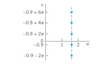
To solve the equation , note first that is the real part of all solutions. Now, since ,

Ans. These are infinitely many solutions (due to the periodicity of ). They lie on the vertical line at a distance from their neighbors.

To summarize: many properties of parallel those of ; an exception is the periodicity of with , which suggested the concept of a fundamental region. Keep in mind that ezis an entire function.(Do you still remember what that means?)

2pi ez

ex ez⫽_{exp z}

䊏

2p x⫽_1.609

ez

z⫽_1.609⫹_0.927i⫾ ₂npi (n⫽_{0, 1, 2,}Á_).

excos y⫽3, exsin y⫽4, cos y⫽0.6, sin y⫽0.8, y⫽0.927.

ex⫽₅

ƒezƒ⫽_ex⫽_{5, x}⫽_{ln 5}⫽_1.609 ez⫽₃⫹_4i

e2e4(cos2 1⫹_sin2

1)⫽_e6_⫽

e(2⫹i)⫹(4ⴚi) e4ⴚi_⫽e4

(cos 1⫺i sin 1)

e2⫹i⫽e2(cos 1⫹i sin 1) ƒe1.4ⴚ1.6i_ƒ⫽e1.4_⫽

4.055, Arg e1.4–0.6i⫽ ⫺0.6.

e1.4ⴚ0.6i_⫽e1.4

(cos 0.6⫺i sin 0.6)⫽4.055(0.8253⫺0.5646i)⫽3.347⫺2.289i ez.

⫺_p⬍y⬉_p

2p w⫽_ez

ez⫹2pi⫽_ez

y

x π

–π

Fig. 336. Fundamental region of the

exponential function ez_{in the z-plane}

1. ez_{is entire.Prove this.}

2–7 Function Values. Find in the form and if zequals

2. 3.

4. 5.

6. _11pi>2 7. 22⫹1_2pi

2⫹_3pi

0.6⫺1.8i

2pi(1⫹_i)

3⫹_4i

ƒezƒ

u⫹iv

ez

8–13 Polar Form.Write in exponential form (6):

8. 9.

10. 11.

12. 13.

14–17 Real and Imaginary Parts.Find Re and Im of

14. eⴚpz 15. exp (z2) 1⫹i

1>(1⫺z)

⫺6.3 1i, 1⫺i

4⫹3i

1n_z

16. 17.

18. TEAM PROJECT. Further Properties of the Ex-ponential Function. (a) Analyticity.Show that is entire. What about ? ? ? (Use the Cauchy–Riemann equations.)

(b) Special values.Find all zsuch that (i) is real, (ii) (iii) .

(c) Harmonic function. Show that is harmonic and find a conjugate. (x2>2⫺_y2_>2)

u⫽exycos

ez⫽_ez

ƒeⴚzƒ⬍_1,

ez ex(cos ky⫹i sin ky)

ez e1>z

ez

exp (z3)

e1>z

SEC. 13.6 Trigonometric and Hyperbolic Functions. Euler’s Formula 633

(d) Uniqueness. It is interesting that is uniquely determined by the two properties

and , where fis assumed to be entire. Prove this using the Cauchy–Riemann equations.

19–22 Equations.Find all solutions and graph some of them in the complex plane.

19. 20.

21. _ez⫽₀ 22. ez⫽ ⫺₂

ez⫽4⫹3i ez⫽1

fr(z)⫽_f(z)

ex

f(x⫹i0) ⫽

f(z)⫽_ez

13.6

Trigonometric and Hyperbolic Functions.

Euler’s Formula

Just as we extended the real to the complex in Sec. 13.5, we now want to extend the familiar realtrigonometric functions to complex trigonometric functions.We can do this by the use of the Euler formulas (Sec. 13.5)

By addition and subtraction we obtain for the realcosine and sine

This suggests the following definitions for complex values

(1)

It is quite remarkable that here in complex, functions come together that are unrelated in real. This is not an isolated incident but is typical of the general situation and shows the advantage of working in complex.

Furthermore, as in calculus we define

(2)

and

(3)

Since is entire, cos zand sin zare entire functions. tan zand sec zare not entire; they are analytic except at the points where cos zis zero; and cot zand csc zare analytic except

ez

sec z⫽ 1

cos z, csc z⫽ 1 sin z. tan z⫽ sin z

cos z, cot z⫽ cos z sin z cos z⫽1_{2 (}eiz⫹eⴚiz), sin z⫽ 1

2i (e

iz_⫺eⴚiz ). z⫽_x⫹_iy: cos x⫽1₂₍eix⫹eⴚix), sin x⫽ 1

2i(e

ix_⫺eⴚix ). eix⫽_{cos x}⫹_{i sin x, e}ⴚix_⫽

cos x⫺_{i sin x.} ez