A Unified View of Kernel k-means, Spectral Clustering and Graph
Cuts
Inderjit Dhillon, Yuqiang Guan and Brian Kulis
University of Texas at Austin
Department of Computer Sciences
Austin, TX 78712
UTCS Technical Report #TR-04-25
February 18, 2005
Abstract
Recently, a variety of clustering algorithms have been proposed to handle data that is not linearly separable. Spectral clustering and kernelk-means are two such methods that are seemingly quite different.
In this paper, we show that a general weighted kernelk-means objective is mathematically equivalent to a
weighted graph partitioning objective. Special cases of this graph partitioning objective include ratio cut, normalized cut and ratio association. Our equivalence has important consequences: the weighted kernel
k-means algorithm may be used to directly optimize the graph partitioning objectives, and conversely,
spectral methods may be used to optimize the weighted kernelk-means objective. Hence, in cases where eigenvector computation is prohibitive, we eliminate the need for any eigenvector computation for graph partitioning. Moreover, we show that the Kernighan-Lin objective can also be incorporated into our framework, leading to an incremental weighted kernel k-means algorithm for local optimization of the
objective. We further discuss the issue of convergence of weighted kernelk-means for an arbitrary graph
affinity matrix and provide a number of experimental results. These results show that non-spectral methods for graph partitioning are as effective as spectral methods and can be used for problems such as image segmentation in addition to data clustering.
Keywords: Clustering, Graph Partitioning, Spectral Methods, Eigenvectors, Kernelk-means, Trace Maxi-mization
1
Introduction
Clustering has received a significant amount of attention as an important problem with many applications, and a number of different algorithms and methods have emerged over the years. In this paper, we unify two well-studied but seemingly different methods for clustering data that is not linearly separable: kernel
k-means and graph partitioning.
The kernelk-means algorithm [1] is a generalization of the standardk-means algorithm [2]. By implicitly mapping points to a higher-dimensional space, kernel k-means can discover clusters that are non-linearly separable in input space. This provides a major advantage over standardk-means, and allows us to cluster points if we are given a positive definite matrix of similarity values.
On the other hand, graph partitioning algorithms focus on clustering nodes of a graph [3, 4]. Spectral methods have been used effectively for solving a number of graph partitioning objectives, including ratio cut [5] and normalized cut [6]. Such an approach has been useful in many areas, such as circuit layout [5] and image segmentation [6].
In this paper, we relate these two seemingly different approaches. In particular, we show that aweighted
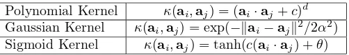
Polynomial Kernel κ(ai,aj) = (ai·aj+c)d
Gaussian Kernel κ(ai,aj) = exp(−kai−ajk2/2α2)
Sigmoid Kernel κ(ai,aj) = tanh(c(ai·aj) +θ)
Table 1: Examples of popular kernel functions
algorithm to locally optimize a number of graph partitioning objectives, and conversely, spectral methods may be employed for weighted kernelk-means. In cases where eigenvector computation is prohibitive (for example, if many eigenvectors of a large matrix are required), the weighted kernelk-means algorithm may be more desirable than spectral methods. In cases where eigenvector computation is feasible, we may use the spectral methods for effective cluster initialization. Subsequently, our analysis implies that by an appropriate choice of weights and kernel, we can use kernelk-means to monotonically improve specific graph partitioning objectives, such as ratio cut, normalized cut, ratio association, and the Kernighan-Lin objective.
Though kernel k-means has the benefit of being able to cluster data that is not linearly separable, it has never really caught on in the research community for specific applications. Some work has been done on scaling kernelk-means to large data sets [7] but the algorithm has not been applied to many real-world problems. Our result provides compelling evidence that weighted kernelk-means is in fact a powerful and useful approach to clustering, especially for graph clustering.
After presenting the equivalence of kernelk-means and graph partitioning objectives, we discuss how to guarantee monotonic convergence of the weighted kernelk-means algorithm for arbitrary graphs. Since the adjacency matrix for an arbitrary graph may not be positive definite, we employ a diagonal shift to enforce positive definiteness. We show that a suitable shift does not change the globally optimal solution to the objective function. We then present experimental results on a number of interesting data sets, including images, text data, and large graphs. We compare various initialization schemes to show that spectral methods are not necessary for optimizing graph partitioning objectives. We show that image segmentation using normalized cuts can be performed without eigenvector computation, and we present the effect of diagonal shifts for text clustering.
A word about our notation. Capital letters such as A, X, and Φ represent matrices. Lower-case bold letters such asa, brepresent vectors. Script letters such asVandE represent sets. We usekakto represent theL2 norm of a vector, andkXk
F for the Frobenius norm of a matrix. Finally,a·bis the inner product
between vectors.
2
Kernel k-means
Given a set of vectorsa1,a2, ...,an, the k-means algorithm seeks to find clusters π1, π2, ...πk that minimize
the objective function:
D({πc}kc=1) =
k
X
c=1
X
ai∈πc
kai−mck2, wheremc =
P
ai∈πcai
|πc|
.
Note that thec-th cluster is denoted by πc, a clustering or partitioning by{πc}kc=1, while the centroid or
mean of clusterπc is denoted by mc.
A disadvantage to standard k-means is that clusters must be separated by a hyperplane; this follows from the fact that squared Euclidean distance is used as the distortion measure. To counter this, kernel
k-means [1] uses a function to map points to a higher-dimensional feature space. Whenk-means is applied in this feature space, the linear separators in the feature space correspond to nonlinear separators in the input space.
The kernelk-means objective can be written as a minimization of:
D({πc}kc=1) =
k
X
c=1
X
ai∈πc
kφ(ai)−mck2, wheremc =
P
ai∈πcφ(ai)
|πc|
If we expand the distance computationkφ(ai)−mck2 in the objective function, we obtain the following:
Thus only inner products are used in the computation of the Euclidean distance between a point and a centroid. As a result, if we are given akernel matrixK, whereKij =φ(ai)·φ(aj), we can compute distances
between points and centroids without knowing explicit representations ofφ(ai) andφ(aj). It can be shown
thatany positive semidefinite matrixKcan be thought of as a kernel matrix [8].
A kernel function κ is commonly used to map the original points to inner products. See Table 1 for commonly used kernel functions;κ(ai,aj) =Kij.
2.1
Weighted kernel
k
-means
We now introduce a weighted version of the kernelk-means objective function, first described in [9]. As we will see later, the weights play a crucial role in showing an equivalence to graph partitioning. The weighted kernelk-means objective function is expressed as:
D({πc}kc=1) =
and the weightswi are non-negative. Note that mc represents the “best” cluster representative since
mc = argminz
X
ai∈πc
wikφ(ai)−zk2.
As before, we compute distances only using inner products, sincekφ(ai)−mck2equals
φ(ai)·φ(ai)−
Using the kernel matrixK, the above may be rewritten as:
Kii−
We now analyze the computational complexity of a simple weighted kernel k-means algorithm presented as Algorithm 1. The algorithm is a direct generalization of standard k-means. As in standard k-means, given the current centroids, the closest centroid for each point is computed. After this, the clustering is re-computed. These two steps are repeated until the change in the objective function value is sufficiently small. It can be shown that this algorithm monotonically converges as long asKis positive semi-definite so that it can be interpreted as a Gram matrix.
It is clear that the bottleneck in the kernelk-means algorithm is Step 2, i.e., the computation of distances d(ai,mc). The first term,Kiiis a constant forai and does not affect the assignment ofai to clusters. The
second term requiresO(n) computation for every data point, leading to a cost of O(n2) per iteration. The
third term is fixed for clusterc, so in each iteration it can be computed once and stored; over all clusters, this takes O(P
c|πc|2) = O(n2) operations. Thus the complexity is O(n2) scalar operations per iteration.
However, for a sparse matrixK, each iteration can be adapted to cost O(nz) operations, where nz is the number of non-zero entries of the matrix (nz = n2 for a dense kernel matrix). If we are using a kernel
functionκto generate the kernel matrix from our data, computingK usually takes timeO(n2m), wherem
is the dimensionality of the original points. If the total number of iterations isτ, then the time complexity of Algorithm 1 isO(n2(τ+m)) if we are given data vectors as input, or O(nz·τ) if we are given a positive
Algorithm 1: Basic Batch Weighted Kernel k-means. Kernel kmeans Batch(K,k,w, tmax,{π(0)c }k
c=1,{πc}kc=1)
Input: K: kernel matrix,k: number of clusters,w: weights for each point,tmax: optional maximum number
of iterations,{πc(0)}kc=1: optional initial clusters
Output: {πc}kc=1: final partitioning of the points
1. If no initial clustering is given, initialize thek clustersπ1(0), ..., πk(0) (i.e., randomly). Sett= 0. 2. For each pointai and every clusterc, compute
d(ai,mc) =Kii−
We now shift our focus to a seemingly very different approach to clustering data: graph partitioning. In this model of clustering, we are given a graphG= (V,E, A), which is made up of a set of verticesV and a set of edgesE such that an edge between two vertices represents their similarity. The affinity matrix A is
|V| × |V|whose entries represent the weights of the edges (an entry ofAis 0 if there is no edge between the corresponding vertices). The graph partitioning problem seeks to partition the graph intokdisjoint partitions or clustersV1, ...,Vk
such that their union isV. A number of different graph partitioning objectives have been proposed and stud-ied, and we will focus on the most prominent ones.
Ratio Association. The ratio association (also called average association) objective [6] aims to maximize within-cluster association relative to the size of the cluster. The objective can be written as
RAssoc(G) = max
Ratio Cut. This objective [5] differs from ratio association in that it seeks to minimize the cut between clusters and the remaining vertices. It is expressed as
RCut(G) = min
Kernighan-Lin Objective. This objective [10] is nearly identical to the ratio cut objective, except that the partitions are required to be of equal size. Although this objective is generally presented for k = 2 clusters, we can easily generalize it for arbitrary k. For simplicity, we assume that the number of vertices
|V|is divisible by k. Then, we write the objective as
Normalized Cut. The normalized cut objective [6, 11] is one of the most popular graph partitioning objectives and seeks to minimize the cut relative to the degree of a cluster instead of its size. The objective is expressed as
N Cut(G) = min V1,...,Vk
k
X
c=1
links(Vc,V \ Vc)
degree(Vc)
.
It should be noted that the normalized cut problem is equivalent to the normalized association problem [11], since links(Vc,V \ Vc) = degree(Vc)−links(Vc,Vc).
General Weighted Graph Cuts/Association. We can generalize the association and cut problems to more general weighted variants. This will prove useful for building a general connection to weighted kernel k-means. We introduce a weight wi for each node of the graph, and for each cluster Vc, define
w(Vc) =Pi∈Vcwi. We generalize the association problem to be:
W Assoc(G) = max V1,...,Vk
k
X
c=1
links(Vc,Vc)
w(Vc)
.
Similarly, for cuts:
W Cut(G) = min V1,...,Vk
k
X
c=1
links(Vc,V \ Vc)
w(Vc)
.
Ratio association is a special case ofW Assocwhere all weights are equal to one (and hence the weight of a cluster is simply the number of vertices in it), and normalized association is a special case where the weight of a nodeiis equal to its degree (the sum of rowiof the affinity matrixA). The same is true forW Cut.
For the Kernighan-Lin objective, an incremental algorithm is traditionally used to swap chains of vertex pairs; for more information, see [10]. For ratio association, ratio cut, and normalized cut, the algorithms used to optimize the objectives involve using eigenvectors of the affinity matrix, or a matrix derived from the affinity matrix. We will discuss these spectral solutions in the next section, where we prove that the W Assocobjective is equivalent to the weighted kernelk-means objective, and thatW Cutcan be viewed as a special case ofW Assoc, and thus as a special case of weighted kernel k-means.
4
Equivalence of the Objectives
At first glance, the two methods of clustering presented in the previous two sections appear to be quite unrelated. In this section, we express the weighted kernelk-means objective as a trace maximization problem. We then show how to rewrite the weighted graph association and graph cut problems identically as matrix trace maximizations. This will show that the two objectives are mathematically equivalent. We discuss the connection to spectral methods, and then show how to enforce positive definiteness of the affinity matrix in order to guarantee convergence of the weighted kernelk-means algorithm. Finally, we extend our analysis to the case of dissimilarity matrices.
4.1
Weighted Kernel
k
-means as Trace Maximization
We first consider the weighted kernelk-means objective, and express it as a trace maximization problem. Letsc be the sum of the weights in clusterc, i.e. sc=Pai∈πcwi. Define then×k matrixZ:
Zic=
( 1
s1c/2 ifai ∈πc,
0 otherwise.
Clearly, the columns ofZare mutually orthogonal as they capture the disjoint cluster memberships. Suppose Φ is the matrix of allφ(a) vectors, andW is the diagonal matrix of the weights. It can then be verified that columniof the matrix ΦW ZZT is equal to the mean vector of the cluster that contains a
Thus, the weighted kernelk-means objective may be written as:
k). Then we write the objective function as:
D({πc}kc=1) =
the minimization of the weighted kernelk-means objective function is equivalent to:
max
˜
Y trace( ˜Y
TW1/2KW1/2Y˜), (3)
where ˜Y is an orthonormaln×kmatrix that is proportional to the square root of the weight matrixW as detailed above.
4.2
Graph Partitioning as Trace Maximization
With this derivation complete, we can now show how each of the graph partitioning objectives may be written as a trace maximization as well.
Ratio Association. The simplest objective to transform into a trace maximization is ratio association. Let us introduce an indicator vectorxc for partitionc, i.e. xc(i) = 1 if clusterc contains vertexi. Then the
ratio association objective equals
size of partitionc, whilexT
cAxc equals the links inside partitionc.
The above can be written as the maximization of trace( ˜XTAX), where the˜ c-th column of ˜X equals ˜x c;
clearly ˜XTX˜ =I
k. It is easy to verify that this maximization is equivalent to the trace maximization for
weighted kernelk-means (Equation 3), where all weights are equal to one, and the affinity matrix is used in place of the kernel matrix.
ratio association in the graph. However, it is important to note that we require the affinity matrix to be positive definite. This ensures that the affinity matrix can be viewed as a kernel matrix and factored as ΦTΦ, thus allowing us to prove that the kernelk-means objective function decreases at each iteration. If
the matrix is not positive definite, then we will have no such guarantee (positive definiteness is a sufficient but not necessary condition for convergence). We will see later in this section how to remove this requirement.
Ratio Cut. Next we consider the ratio cut problem:
min
we can easily verify that the objective function can be rewritten as:
min
where ˜xc is defined as before. The matrix D−A is known as the Laplacian of the graph, so we write
it as L. Hence, we may write the problem as a minimization of trace( ˜XTLX˜). We convert this into
a trace maximization problem by considering the matrix I−L, and noting that trace( ˜XT(I−L) ˜X) =
trace( ˜XTX)˜ −trace( ˜XTLX˜). Since ˜X is orthonormal, trace( ˜XTX˜) =k, so maximizing trace( ˜XT(I−L) ˜X)
is equivalent to the minimization of trace( ˜XTLX˜).
Putting this all together, we have arrived at an equivalent trace maximization problem for ratio cut: minimizing the ratio cut for the affinity matrix is equivalent to maximizing trace( ˜XT(I−L) ˜X). Once again,
this corresponds to unweighted kernelk-means, except that the matrixKisI−L. We will see how to deal with the positive definiteness issue later.
Kernighan-Lin Objective. The Kernighan-Lin (K-L) graph partitioning objective follows easily from the ratio cut objective. For the case of K-L partitioning, we maintain equally sized partitions, and hence the only difference between the ratio cut and K-L partitioning is that thexcindicator vectors are constrained to
be of size|V|/k. If we start with equally sized partitions, an incremental weighted kernelk-means algorithm (where we only consider swapping points, or chains of points, that improve the objective function) can be run to simulate the Kernighan-Lin algorithm.
Normalized Cut. We noted earlier that the normalized cut problem is equivalent to the normalized association problem; i.e., the problem can be expressed as:
max
Then, if the matrixK is positive definite, we have a way to iteratively minimize the normalized cut using weighted kernelk-means. Note that the seemingly simpler choice of W =D−1 and K=A does not result
in a direct equivalence since ˜Y is a function of the partition and the weights.
Our analysis easily extends to theW Cutproblem. Using the same notation forW andxc, we write the
problem as:
W Cut(G) = min
k
X
c=1
xT
c(D−A)xc
xT cWxc
= min
k
X
c=1
˜
xTcL˜xc
= min
Y trace(Y
TW−1/2LW−1/2Y).
TheW Cutproblem can be expressed asW Assocby noting that
trace(YTW−1/2(W −L)W−1/2Y) =k−trace(YTW−1/2LW−1/2Y),
and therefore the W Cut problem is equivalent to maximizing trace(YTW−1/2(W −L)W−1/2Y). Hence,
optimizingW Assoc on the graph affinity matrixW−Lis equivalent to optimizingW CutonA. We observed that ˜Y from the previous section is an orthornormal matrix; in particular,
˜ Yic=
( w1/2
i
s1c/2 ifi∈πc,
0 otherwise,
where sc =xTcWxc. It is easy to see that the matrix Y in this section is idential to ˜Y from Section
IV-A. Then the trace maximization for weighted kernelk-means equals trace( ˜YTW−1/2AW−1/2Y˜), which is
exactlythe trace maximization for weighted graph association from Equation 4. In the other direction, given a kernel matrixK and a weight matrixW, define an affinity matrixA=W KW to obtain the equivalence. We see that it is easy to map from one problem to the other.
4.3
The Spectral Connection
A standard result in linear algebra [12] states that if we relax the trace maximizations in Equations 3 and 4 such thatY is an arbitrary orthonormal matrix, then the optimal Y is of the formVkQ, whereˆ Vk consists
of the leading k eigenvectors of W1/2KW1/2 and ˆQ is an arbitrary k×k orthogonal matrix. As these
eigenvectors are not indicator vectors, we must then perform postprocessing on the eigenvectors to obtain a discrete clustering of the points, which we discuss in Section 5.
Using this result, spectral algorithms that compute and use the leading k eigenvectors of W1/2KW1/2
have almost exclusively been used to optimize graph partitioning objectives, such as ratio cut [5] and nor-malized cut [6, 11]. In the same spirit, spectral algorithms have recently been used for data clustering [13]. However, our equivalence shows that spectral solutions are not necessary.
Before we proceed further by validating our theoretical results with experiments, we show how to enforce positive definiteness for graph partitioning problems.
4.4
Enforcing Positive Definiteness
For weighted graph association, we define a matrix K =W−1AW−1 to map to weighted kernelk-means.
However, when A is an arbitrary adjacency matrix, W−1AW−1 need not be positive definite and hence
Algorithm 1 will not necessarily converge. In this section, we show how to avoid this problem by introducing a diagonal shift toK. Furthermore, we discuss how such a diagonal shift affects the practical performance of the weighted kernelk-means algorithm.
Given A, define K′
= σW−1+W−1AW−1, where σ is a constant large enough to ensure that K′ is positive definite. Since W−1 is a diagonal matrix, adding σW−1 adds positive entries to the diagonal of
W−1AW−1. If we plug K′
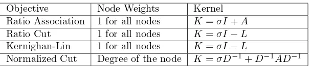
Objective Node Weights Kernel Ratio Association 1 for all nodes K=σI+A Ratio Cut 1 for all nodes K=σI−L Kernighan-Lin 1 for all nodes K=σI−L
Normalized Cut Degree of the node K=σD−1+D−1AD−1
Table 2: Popular graph partitioning objectives and corresponding weights and kernels given affinity matrix A
Hence, maximizing ˜Y usingK′
is identical to that of the weighted association problem (Equation 4), except thatK′
is constructed to be positive definite. Running weighted kernelk-means onK′
results in monotonic optimization of the weighted association objective.
A similar approach can be used for the weighted cut problem. We showed earlier howW Cuton affinity matrix A is equivalent to W Assoc on W −L. Hence, if we let A′
= W −L, it follows that defining K′
= σW−1+W−1A′
W−1 for large enough σ gives us a positive definite kernel for the weighted kernel
k-means algorithm. In Table 2, the weights and kernels for several graph objectives are summarized. However, although adding a diagonal shift does not change the global optimal clustering, it is important to note that adding too large a shift may result in a decrease in quality of the clusters produced by Algorithm 1. To illustrate this, consider the case of ratio association, where the node weights equal 1. Given an affinity matrixA, we define a kernelK=σI+A for sufficiently largeσ. In the assignment step of Algorithm 1, we consider the distance from points to all centroids.
First, using Equation 2, let us calculate the distance from ai to the centroid of πc given this σ shift,
assuming thatai is in πc:
Secondly, we calculate this distance assuming thatai is not inπc:
Kii+σ−
0 0.2 0.4 0.6 0.8 1
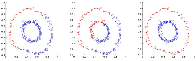
Figure 1: Results using three different cluster initialization methods. Left: random initialization; Middle: spectral initialization; Right: random initialization on a kernel withσ=−1
It is natural to ask the following question: since weighted kernelk-means can perform poorly with a large positiveσshift, what happens when we add a negativeσshift? This is akin to reducing “self-similarity” of points, thereby magnifying the similarity to other points. Clearly, we cannot theoretically guarantee that the algorithm will always converge, since the kernel matrix will be indefinite. However, we have seen that, in practice, kernelk-means often converges and in fact, yields superior local opitmal solutions when run with a negative shift. For example, consider a data set consisting of two circles as shown in Figure 1. We used an exponential kernel to generate an affinity matrix (2α2 = 0.05). Then we clustered the points in three
different ways: a) kernel k-means with random initialization, b) kernel k-means using a ratio association spectral clustering algorithm for cluster initialization, c) kernelk-means using random initialization and a kernel with aσ=−1 shift. Figure 1 shows that, in this simple case, the negative shift is the only algorithm to achieve perfect clustering results. Thus, it appears that for some graph partitioning problems, it may be better to run weighted kernelk-means using an indefinite matrix, at least as an initialization step; as the algorithm may not converge, running kernelk-means for a set number of iterations on an indefinite matrix is a strong initialization technique. A good choice forσis one that makes the trace of the kernel matrix equal to zero.
4.5
Distance Matrices and Graph Cuts
In many applications, distance (or dissimilarity) matrices arise naturally instead of similarity matrices. We now take a short digression to expand our analysis to this case.
It is well known ([14], Sec. 10.7.2) that the standardk-means objective function to be minimized may be written in the following way:
k
This is just the minimum ratio association problem on the graph defined by the distance matrix E (as opposed to the maximization problem in Equation 4 for a graph affinity matrix). Given such a distance matrix, we may like to be able to locally optimize thek-means objective function, even if we do not have an explicit coordinate representation of the points.
We can easily extend the analysis we gave earlier for this setting. Minimizing the weighted association, a problem we will callM inW Assoc, is expressed as:
M inW Assoc(G) = minimize trace(YTW−1/2EW−1/2Y).
The only difference betweenM inW AssocandW Associs the minimization. The same trick that we used for W Cutapplies here: lettingE′ =σW−W−1/2EW−1/2results in an equivalent trace maximization problem.
The value ofσ is chosen to be sufficiently large such thatE′ is positive definite (and hence E need not be positive definite).
For maximizing the weighted cut, we note thatM axW Cut is written as:
M axW Cut(G) = maximize trace(YTW−1/2LW−1/2Y).
This is equivalent to W Assoc, with the Laplacian L of E, in place of A. Again, a diagonal shift may be necessary to enforce positive definiteness.
Thus, handling minimum association and maximum cut problems on dissimilarity matrices follows easily from our earlier analysis.
5
Putting it All Together
In this section, we touch on a few important remaining issues. As mentioned earlier, spectral methods can be used as an initialization step for graph partitioning objectives. We discuss two methods for obtaining a discrete clustering from eigenvectors, and then generalize these methods to obtain initial clusterings for weighted kernelk-means.
To further improve the quality of results obtained using kernel k-means, we examine the use of local search. Local search is an effective way to avoid local optima, and can be implemented efficiently in kernel
k-means.
Combining both of these strategies, we arrive at our final, enhanced algorithm for weighted kernelk-means in Section 5.3.
5.1
From Eigenvectors to a Partitioning
Bach and Jordan Postprocessing. DenoteU as then×kmatrix of thekleading eigenvectors ofW1/2KW1/2,
obtained by solving the relaxed trace maximization for weighted kernel k-means. The Bach and Jordan method [15] was presented to obtain partitions from eigenvectors in the context of minimizing the normalized cut. Below, we generalize this method to cover all weighted kernelk-means cases. The method compares the subspace spanned by the columns ofU with the subspace spanned by the columns of Y, the desiredn×k orthonormal indicator matrix. We seek to find aY with the given structure that minimizeskU UT−Y YTk2
F,
thus comparing the orthogonal projection corresponding to the subspaces spanned byU andY. We rewrite the minimization as:
kU UT −Y YTk2F
= trace(U UT +Y YT −U UTY YT−Y YTU UT) = 2k−2trace(YTU UTY).
Hence, the task is equivalent to maximizing trace(YTU UTY). The equivalence of this step to weighted
kernelk-means can be made precise as follows: the kernel k-means objective function can be written as a maximization of trace(YTW1/2KW1/2Y). SinceY is a function of the partition and the weightsW, we set
K = W−1/2U UTW−1/2, and the objective function for weighted kernelk-means with this K is therefore
written as a maximization of trace(YTU UTY). Hence, we may use weighted kernel k-means to obtain
partitions from the eigenvectors.
To summarize, after obtaining the eigenvector matrix U, we can iteratively minimize kU UT −Y YTk2
F
by running weightedk-means on the rows ofW−1/2U, using the original weights. Note: we do not have to
Yu and Shi Postprocessing. An alternative method for spectral postprocessing of normalized cuts was pro-posed by Yu and Shi [11]. We briefly describe and generalize this method below.
As before, letU be then×kmatrix of the kleading eigenvectors ofW1/2KW1/2. GivenU, the goal of
this method is to find the 0-1 partition matrixX which is closest to U, over all possible orthogonal k×k orthogonal matricesQ. This may be accomplished as follows. Form the matrix X∗
, which is U with the rows normalized to haveL2 norm 1. Given this matrix, we seek to find a true partition matrix that is close
toX∗
. We therefore minimize kX−X∗
Qk2 over all partition matricesX and square orthonormal Q. An
alternate minimization procedure is then used to locally optimize this objective. Weights play no role in the procedure.
The alternate minimization procedure is performed as follows: to minimize kX−X∗Qk2, where Q is
fixed, we compute
Xil=
½
1 ifl= argmaxk(X∗Q)ik
0 otherwise
for all i. Similarly, when X is fixed, we compute the optimal Q as follows: compute the singular value decomposition ofXTX∗=UΣVT, and setQ=V UT. We alternate updatingX andQuntil convergence.
We note that we may express the Yu and Shi objective askX−X∗Qk2=kX∗−XQTk2. The standard
k-means objective function can be expressed as a minimization of kA−XBk2, where A is the input data
matrix,X is a 0-1 partition matrix, andB is an arbitrary matrix. Thus, the Yu and Shi objective is nearly identical to k-means, with the only difference arising from the restriction on Qthat it be an orthonormal matrix.
5.2
Local Search
A common problem when running standard batchk-means or batch kernelk-means is that the algorithm has the tendency to be trapped into qualitatively poor local optima.
An effective technique to counter this issue is to use local search [16] during the algorithm by incorporating incremental weighted kernelk-means into the standard batch algorithm. A step of incremental kernel k -means attempts to move a single point from one cluster to another in order to improve the objective function. For a single move, we look for the move that causes the greatest decrease in the value of the objective function. For a chain of moves, we look for a sequence of such moves. The set of local optima using local search is a superset of the local optima using the batch algorithm. Often, this enables the algorithm to reach a much better local optima. Details can be found in [16].
It has been shown in [16] that incrementalk-means can be implemented efficiently. Such an implementa-tion can be easily be extended to weighted kernelk-means. In practice, we alternate between doing standard batch updates and incremental updates.
The Kernighan-Lin objective can also be viewed as a special case of the weighted kernelk-means objective (the objective is the same as ratio cut except for the cluster size restrictions), but running weighted kernel
k-means provides no guarantee about the size of the partitions. We may still optimize the Kernighan-Lin objective, using a local search-based approach based on swapping points: if we perform only local search steps via swaps during the weighted kernelk-means algorithm, then cluster sizes remain the same. An approach to optimizing Kernighan-Lin would therefore be to run such an incremental kernelk-means algorithm using chains of swaps. This approach is very similar to the usual Kernighan-Lin algorithm [10]. Moreover, spectral initialization could be employed, such that during spectral postprocessing, an incrementalk-means algorithm is used on the eigenvector matrix to obtain initial clusters.
5.3
Final Algorithm
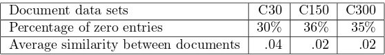
Document data sets C30 C150 C300 Percentage of zero entries 30% 36% 35% Average similarity between documents .04 .02 .02
Table 3: Self-similarity of documents is much higher than similarity between different documents
Data sets C30 C150 C300 Average NMI (σ= 0) .075 .02 .11 Average NMI (σ=−1) .6 .64 .62
Table 4: Comparison of NMI values achieved by Algorithm 1 before and afterσshift
could easily be added to this list. After we obtain initial clusters, we makeK positive definite by adding to the diagonal. Finally, we oscillate between running batch weighted kernelk-means and incremental weighted kernelk-means (local search) until convergence.
6
Experimental Results
In previous sections, we presented a unified view of graph partitioning and weighted kernelk-means. Now we experimentally illustrate some implications of our results. Specifically, we show that 1) a negative σ shift on the diagonal of the kernel matrix can significantly improve clustering results in document clustering applications; 2) graph partitioning using the final algorithm of Section 5.3 gives an improvement over spectral methods, when spectral initialization is used, and in some cases, METIS initialization is as effective as spectral initialization; 3) normalized cut image segmentation can be performed without the use of eigenvectors.
Our algorithms are implemented in MATLAB. When random initialization is used, we report the average results over 10 runs. All the experiments are performed on a Linux machine with 2.4GHz Pentium IV processor and 1GB main memory.
6.1
Document clustering
In document clustering, it has been observed that when similarity of documents with the cluster that they belong to is dominated by their self-similarity (similarity of documents with themselves), clustering algo-rithms can generate poor results [16]. In a kernel matrix that describes pairwise similarity of documents, a negativeσshift on the diagonal, as we discussed in Section 6.4, reduces the self-similarity of documents. We show that this can improve performance as compared to no negative shift on text data.
The three document sets that we use are C30, C150 and C300 [16]. They are created by an equal sampling of theMEDLINE,CISI, andCRANFIELDcollections (available from ftp://ftp.cs.cornell.edu/pub/smart).
The sets C30, C150 and C300 contain 30, 150 and 300 documents and are of 1073, 3658 and 5577 dimensions, respectively. The document vectors are normalized to haveL2 norm 1.
Since we know the underlying class labels, to evaluate clustering results we can form a confusion matrix, where entry (i, j),n(ij)gives the number of documents in clusteriand classj. From such a confusion matrix,
we compute normalized mutual information (NMI) [9] as
2Pk
wherecis the number of classes,ni is the number of documents in clusteri,n(j)is the number of documents
in classj,H(π) =−Pk
. A high NMI value indicates that the clustering and true class label match well.
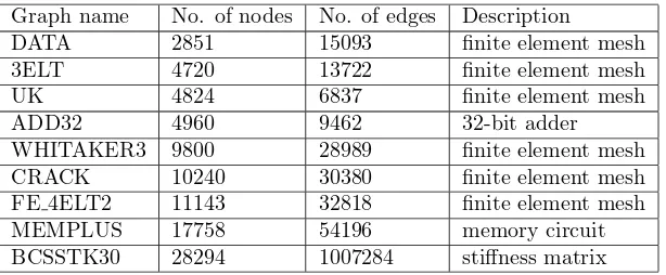
Graph name No. of nodes No. of edges Description
DATA 2851 15093 finite element mesh 3ELT 4720 13722 finite element mesh
UK 4824 6837 finite element mesh
ADD32 4960 9462 32-bit adder
WHITAKER3 9800 28989 finite element mesh CRACK 10240 30380 finite element mesh FE 4ELT2 11143 32818 finite element mesh MEMPLUS 17758 54196 memory circuit BCSSTK30 28294 1007284 stiffness matrix
Table 5: Test graphs
0.02 and 0.04. Compared to a self-similarity of 1, the similarities between different documents are much lower. We run Algorithm 1 with random initialization 100 times on the three Gram matrices. 97 out of 100 runs stop immediately after initialization, resulting in very poor NMI values. The relatively high self-similarity makes each document much closer to its own cluster than to other clusters and therefore no documents are moved after initialization. A similar observation was made in [16], where local search was used to fix this problem. Here we apply the negativeσshift strategy by subtracting 1 from every diagonal entry of the Gram matrices (note that the average of the trace of the Gram matrix equals 1). We then run Algorithm 1 on the modified matrices 100 times, and observe that documents move among clusters after random initialization in all runs, resulting in much higher average NMI values. Table 4 shows the comparisons of averaged NMI values over 100 random runs before and after we do the σ shift. Perfect clustering results are achieved for all three data sets if we add local search to our algorithm. In all the experiments in the following two subsections, we add local search to Algorithm 1 to improve the final clustering.
6.2
Graph partitioning
As we showed in earlier sections, weighted kernelk-means can be used to optimize various objectives, such as ratio association or normalized association, given the proper weights. Moreover, the algorithm takes an initial clustering and improves the objective function value. In our experiments in this subsection, we evaluate improvement in ratio association and normalized association values by Algorithm 1 using three different initialization methods: random, METIS and spectral. Randomly assigning a cluster membership to each data point is simple but often gives poor initial objective function value. We measure how much our algorithm improves the poor initial objective values and use results from random initialization as a baseline in our comparisons. METIS is a fast, multi-level graph partitioning algorithm which seeks balanced partitions while minimizing the cut value. We use the output of METIS to initialize Algorithm 1. Spectral algorithms are often used for initialization because they produce clusterings which are presumably ‘close’ to the global optimal solution. We use Yu and Shi’s method described in Section 5.1 for spectral initialization. Table 5 lists 9 test graphs from various sources and different application domains. Some of them are benchmark matrices used to test METIS. All the graphs are downloaded fromhttp://staffweb.cms.gre.
ac.uk/~c.walshaw/partition/.
data 3elt uk add32 whitaker3 crack fe_4elt2 memplus 0
50 100 150 200 250 300 350
Ratio Association value
initial (random) final (random) initial (METIS) final (METIS) initial (spectral) final (spectral)
data 3elt uk add32 whitaker3 crack fe_4elt2 memplus 0
100 200 300 400 500 600
Ratio Association value
data 3elt uk add32 whitaker3 crack fe_4elt2 memplus 0
100 200 300 400 500 600 700 800 900 1000
Ratio Association value
Figure 2: Plots of initial and final ratio association values for 32 clusters (left), 64 clusters (middle) and 128 clusters (right) generated using random, METIS and spectral initialization
32 clusters 64 clusters 128 clusters Graph Rand METIS Spec Rand METIS Spec Rand METIS Spec DATA 265.9 297.5 317.8 506.7 543.1 566.5 921.1 956.4 976.4 3ELT 125.5 171.9 172.3 246.8 327.1 328.4 471.4 608.5 612.8 UK 15.6 86.4 87.7 32.3 168.8 171.4 60.9 323.3 328.7 ADD32 109.2 126.1 119.1 215.5 259.7 252.4 411.4 433.5 471.8 WHITAKER3 123.7 177.4 177.9 239.2 342.4 344.4 469.0 653.1 654.8 CRACK 134.2 177.9 178.3 261.5 344.5 346.3 509.5 656.1 667.7 FE 4ELT2 125.8 178.4 176.2 246.1 345.5 344.4 479.9 662.0 663.5 MEMPLUS 215.5 240.5 239.8 315.3 356.3 343.0 507.6 556.3 505.0 BCSSTK30 1710.7 2050.5 2053.4 3263.2 3862.8 3900.9 6123.3 6922.7 7101.7
Table 6: Final ratio association values achieved using random, metis and spectral initialization
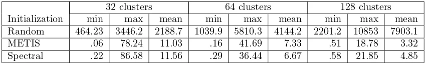
32 clusters 64 clusters 128 clusters Initialization min max mean min max mean min max mean Random 464.23 3446.2 2188.7 1039.9 5810.3 4144.2 2201.2 10853 7903.1 METIS .06 78.24 11.03 .16 41.69 7.33 .51 18.78 3.32 Spectral .22 86.58 11.56 .29 36.44 6.67 .58 21.85 4.85
data 3elt uk add32 whitaker3 crack fe_4elt2 memplus bcsstk30 0
5 10 15 20 25 30 35
Normalized association value
initial (random) final (random) initial (METIS) final (METIS) initial (spectral) final (spectral)
data 3elt uk add32 whitaker3 crack fe_4elt2 memplus bcsstk30 0
10 20 30 40 50 60 70
Normalized association value
data 3elt uk add32 whitaker3 crack fe_4elt2 memplus bcsstk30 0
20 40 60 80 100 120
Normalized association value
Figure 3: Plots of initial and final normalized association values of 32 clusters (left), 64 clusters (middle) and 128 clusters (right) generated using random, METIS and spectral initialization
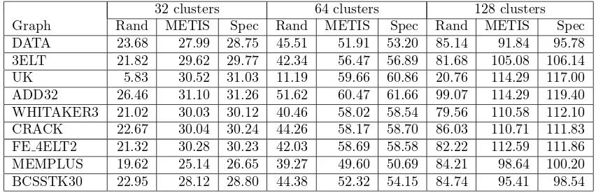
32 clusters 64 clusters 128 clusters Graph Rand METIS Spec Rand METIS Spec Rand METIS Spec DATA 23.68 27.99 28.75 45.51 51.91 53.20 85.14 91.84 95.78 3ELT 21.82 29.62 29.77 42.34 56.47 56.89 81.68 105.08 106.14 UK 5.83 30.52 31.03 11.19 59.66 60.86 20.76 114.29 117.00 ADD32 26.46 31.10 31.26 51.62 60.47 61.66 99.07 114.29 119.40 WHITAKER3 21.02 30.03 30.12 40.46 58.02 58.54 79.56 110.58 112.10 CRACK 22.67 30.04 30.24 44.26 58.17 58.70 86.03 110.71 111.83 FE 4ELT2 21.32 30.28 30.23 42.03 58.69 58.58 82.22 112.59 111.86 MEMPLUS 19.62 25.14 26.65 39.27 49.60 50.69 84.21 98.64 100.20 BCSSTK30 22.95 28.12 28.80 44.38 52.32 54.15 84.74 95.41 98.54
Table 8: Final normalized association values achieved using random, metis and spectral initialization
or spectral initialization, Algorithm 1 increases the ratio association value of MEMPLUS by 78-87% in the case of 32 clusters, 36-42% in case of 64 clusters and 19-22% in case of 128 clusters, respectively. Spectral methods are used in many applications because they generate high-quality clustering results. However, computing a large number of eigenvectors is computationally expensive and sometimes convergence is not achieved by the MATLAB sparse eigensolver. We see that for ratio association, our algorithm, with fast initialization using METIS, achieves comparable clustering results without computing eigenvectors at all.
32 clusters 64 clusters 128 clusters Initialization min max mean min max mean min max mean Random 485.71 2551.37 1964.35 1011.5 5191.99 3965.83 2051.28 9415.05 7912.3
Metis .08 10.49 1.55 .27 15.14 2.37 .6 21.93 3.55
Spectral .1 1.41 .42 .17 8.32 1.54 .33 9.83 1.98
Table 9: Min, max and mean percentage increase in normalized association over the 9 graphs listed in Table 5 that is generated by our algorithm using random, metis or spectral initialization
1 2 3 4 5 6 7 8 9 30.22
30.24 30.26 30.28 30.3 30.32 30.34 30.36
Iteration count
Normalized association value
batch local search
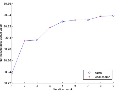
Figure 4: One run of the final algorithm using spectral initialization on graph FE 4ELT2; 32 clusters
clusters. This underlines the value of using weighted kernel k-means to improve graph partitioning results even when a sophisticated algorithm, such as spectral graph partitioning, is used.
The effect of local search is illustrated in Figure 4, where a local search chain of length 20 is represented as one iteration step. The plot shows that the local search steps help to keep increasing the normalized association value when the batch algorithm gets stuck at local optima.
6.3
Image segmentation
Normalized cuts are often used for image segmentation [11], though generally eigenvectors of a large affinity matrix must be computed. This may be quite computationally expensive, especially if many eigenvectors are needed. In addition, Lanczos type algorithms can sometimes fail to converge in a pre-specified number of iterations (this occurred in some of our MATLAB runs on the image data set). However, using Algorithm 1, we can minimize normalized cuts without computing eigenvectors at all. Figure 5 shows the segmentation of a sample image done by Algorithm 1, where three clusters are computed. Some preprocessing was done on the image using code obtained fromhttp://www.cs.berkeley.edu/~stellayu/code.html.
7
Related Work
Figure 5: Segmentation of image. The leftmost plot is the original image and each of the 3 plots to the right of it is a component (cluster) — body, feet and tail.
Our results generalize this work to the case when kernels are used for non-linear separators, plus we treat the weighted version of kernelk-means which is a powerful extension that allows us to encompass various spectral clustering objectives such as minimizing the normalized cut.
In [15], the authors hint at a way to run an iterative algorithm for normalized cuts, though their algorithm considers the factorization of a semi-definite matrixK such thatK=GGT. This would lead to ak-means
like formulation, though the factorization could take time O(n3), which would be much slower than our
approach; neither [15] nor [11] consider kernelk-means. Our methods, which stem from kernelk-means, do not need the expensiveO(n3) factorization of the kernel matrix.
The notion of using a kernel to enhance thek-means objective function was first described in [1]. This paper also explored other uses of kernels, most importantly in nonlinear component analysis. Kernel-based learning methods have appeared in a number of other areas in the last few years, especially in the context of support vector machines [8].
Some research has been done on reformulating the kernelk-means objective function. In [19], the objective function was recast as a trace maximization, though their work differs from ours in that their proposed clustering solution did not use any spectral analysis. Instead, they developed an EM-style algorithm to solve the kernelk-means problem.
A recent paper [20] discusses the issue of enforcing positive definiteness for clustering. The focus in [20] is on embedding points formed from a dissimilarity matrix into Euclidean space, which is equivalent to forming a positive definite similarity matrix from the data. Their work does not touch upon the equivalence of various clustering objectives.
Our earlier paper [9] introduced the notion of weighted kernelk-means and showed how the normalized cut objective is a special case. This paper substantially extends the analysis of the earlier paper by discussing a number of additional objectives, such as ratio cut and ratio association, and the issue of enforcing positive definiteness to handle arbitrary graph affinity matrices. We also provide experimental results on large graphs and image segmentation.
8
Conclusion
Until recently, kernelk-means has not received a significant amount of attention among researchers. How-ever, by introducing a more general weighted kernelk-means objective function, we have shown how several important graph partitioning objectives follow as special cases. In particular, we considered ratio association, ratio cut, the Kernighan-Lin objective, and normalized cut. We generalized these problems to weighted asso-ciation and weighted cut objectives, and showed that weighted cut can be expressed as weighted assoasso-ciation, and weighted association can be expressed as weighted kernelk-means.
Moreover, we have discussed the issue of enforcing positive definiteness. As a result of our analysis, we have shown how cluster initialization using a negativeσshift encourages points to move around during the clustering algorithm, and sometimes gives results comparable to spectral initialization. We also showed how each of the graph partitioning objectives can be written in a way that weighted kernelk-means is guaranteed to monotonically improve the objective function at every iteration.
In the future, we would like to develop a more efficient method for locally optimizing the kernelk-means objective. In particular, we may be able to use ideas from other graph partitioning algorithms, such as METIS, to speed up weighted kernelk-means when using large, sparse graphs. We showed how initialization using METIS works nearly as well as spectral initialization. A more general graph partitioning algorithm that works like METIS for the weighted kernel k-means objective function would prove to be extremely useful in any domain that uses graph partitioning.
Finally, we presented experimental results on a number of data sets. We showed how image segmentation, which is generally performed by normalized cuts using spectral methods, may be done without computing eigenvectors. We showed that for large, sparse graphs, partitioning the graph can be done comparably with or without spectral methods. We have provided a solid theoretical framework for unifying two methods of clustering, and we believe that this will lead to significant improvements in the field of clustering.
References
[1] B. Sch¨olkopf, A. Smola, and K.-R. M¨uller, “Nonlinear component analysis as a kernel eigenvalue prob-lem,”Neural Computation, vol. 10, pp. 1299–1319, 1998.
[2] J. MacQueen, “Some methods for classification and analysis of multivariate observations,” inProceedings of the Fifth Berkeley Symposium on Math., Stat. and Prob., 1967, pp. 281–296.
[3] W. E. Donath and A. J. Hoffman, “Lower bounds for the partitioning of graphs,”IBM J. Res. Devel-opment, vol. 17, pp. 422–425, 1973.
[4] K. M. Hall, “An r-dimensional quadratic placement algorithm,” Management Science, vol. 11, no. 3, pp. 219–229, 1970.
[5] P. Chan, M. Schlag, and J. Zien, “Spectralk-way ratio cut partitioning,”IEEE Trans. CAD-Integrated Circuits and Systems, vol. 13, pp. 1088–1096, 1994.
[6] J. Shi and J. Malik, “Normalized cuts and image segmentation,” IEEE Trans. Pattern Analysis and Machine Intelligence, vol. 22, no. 8, pp. 888–905, August 2000.
[7] R. Zhang and A. Rudnicky, “A large scale clustering scheme for kernelk-means,” in ICPR02, 2002, pp. 289–292.
[8] N. Cristianini and J. Shawe-Taylor,Introduction to Support Vector Machines: And Other Kernel-Based Learning Methods. Cambridge, U.K.: Cambridge University Press, 2000.
[9] I. Dhillon, Y. Guan, and B. Kulis, “Kernelk-means, spectral clustering and normalized cuts,” inProc. 10th ACM KDD Conference, 2004.
[10] B. Kernighan and S. Lin, “An efficient heuristic procedure for partitioning graphs,” The Bell System Technical Journal, vol. 49, no. 2, pp. 291–307, 1970.
[11] S. X. Yu and J. Shi, “Multiclass spectral clustering,” inInternational Conference on Computer Vision, 2003.
[12] G. Golub and C. Van Loan,Matrix Computations. Johns Hopkins University Press, 1989.
[13] A. Y. Ng, M. Jordan, and Y. Weiss, “On spectral clustering: Analysis and an algorithm,” inProc. of NIPS-14, 2001.
[15] F. Bach and M. Jordan, “Learning spectral clustering,” inProc. of NIPS-17. MIT Press, 2004.
[16] I. S. Dhillon, Y. Guan, and J. Kogan, “Iterative clustering of high dimensional text data augmented by local search,” inProceedings of The 2002 IEEE International Conference on Data Mining, 2002, pp. 131–138.
[17] G. Karypis and V. Kumar, “A fast and high quality multilevel scheme for partitioning irregular graphs,”
SIAM J. Sci. Comput., vol. 20, no. 1, pp. 359–392, 1999.
[18] H. Zha, C. Ding, M. Gu, X. He, and H. Simon, “Spectral relaxation fork-means clustering,” inNeural Info. Processing Systems, 2001.
[19] M. Girolami, “Mercer kernel based clustering in feature space,”IEEE Transactions on Neural Networks, vol. 13, no. 4, pp. 669–688, 2002.