11 (2000) 317 – 336
An integration of Schumpeterian and classical
theories of growth and distribution
Reiner Franke *
Department of Economics,Uni6ersity of Bremen,28334Bremen,Germany Accepted 30 September 1999
Abstract
Starting out from a classical perspective on income distribution and growth, the paper reconsiders this issue in the framework of a basic (deterministic) Schumpeterian model with ongoing technical change. On a long-run equilibrium path of this economy, the forces of technological innovation and diffusion balance such that always various techniques of different efficiencies coexist. A consequence of this equilibrium notion is that prices and income distribution can no longer be determined independently of quantities, and that distribution is affected by behavioural parameters beyond the scope of the classical analysis. On the other hand, wages and profits continue to be inversely related. It is also indicated that the present approach casts new light on the internal consistency of the Marxian law of the falling rate of profit. © 2000 Elsevier Science B.V. All rights reserved.
JEL classification:O30; O40
Keywords:Technological innovation and diffusion; Schumpeterian long-run equilibrium; Wave train; Wage-profit frontier; Falling rate of profit
www.elsevier.nl/locate/econbase
1. Introduction
Classical and neoclassical theories of growth and income distribution have one thing in common: even in models with technical progress, both theories suppose that all firms have free access to the most efficient technological knowledge, or that the competitive process works so fast as to drive old production methods out of the
* Fax: +49-421-2184336.
E-mail address:[email protected] (R. Franke).
market immediately when a new and more profitable technique enters the stage. Apart from the wide gap between this idealized world and the industrial structure to be observed in reality, the assumption raises a fundamental problem at the theoretical level, namely, that there would be no one within the system
who has any motivation to change the reached position. Strictly speaking, the long-run equilibrium notion of the classical and neo-classical theory, if it is to apply to a capitalist economy, is a contradiction in terms (Metcalfe, 1997, p. 6).
With respect to the dynamic character of a capitalist economy, a Schumpeterian view seems more meaningful. What Schumpeter envisaged as ‘the essential fact about capitalism’ (Schumpeter, 1950, p. 83) is the process of ‘creative destruction’, a process that ‘incessantly revolutionizes the economic structure from within, incessantly destroying the old one, incessantly creating a new one’. According to this view economic theory should seriously take into account ‘the ceaselessly changing pattern of economic activity, expressed over time by the emergence of new activities, the demise of existing ones and the changing relative importance of those that currently compete for markets’ (Metcalfe, 1997, p. 6).
Limiting the discussion to technical change and the introduction of unambigu-ously more efficient production methods in a one-good world, these features can already be captured by a Schumpeterian prototype model as it has been put forward by Iwai (1984). The basic forces are here technological diffusion and innovation. Their interplay suggests another and more advanced equilibrium no-tion, which can be described as a balance of the centripetal forces of diffusion with their tendency toward the technological frontier, and the centrifugal forces of a never ceasing inflow of new technological knowledge. Since diffusion is gradual and not instantaneous, the economy has in each period a non-degenerate spectrum of coexisting techniques, a multitude of diverse production methods with different efficiencies. As the dynamic process unfolds, the least productive vintages are wiped out through evolutionary pressure, while at the other end of the spectrum new and more profitable production methods are continuously added.
The present paper focusses on this equilibrium notion and its direct implications. To make the argument as simple as possible, technical progress and also the rates of diffusion are assumed to be exogenous1. If furthermore the innovations improve uniformly and are introduced deterministically at regular intervals of lengthT, the economy is in long-run equilibrium when the capacity shares of the techniques reproduce themselves over time — only at an increasing technological scale. This means more precisely that the role of techniqueiat timetis taken over by its more
productive successori+1 at time t+T. Such a smooth evolution of the economy is called awa6e train2.
Of course, proponents of classical and neo-classical theories are aware of the methodological criticism mentioned above. They argue that their equilibrium concept is nevertheless a convenient instrument that since long has proved worth-while to study growth and income distribution. The sketchy remarks in the preceding paragraph indicate that alternative modelling devices are available. They can incorporate basic aspects of the Schumpeterian vision and are thus able to overcome (to some extent) the basic methodological problem of the orthodox theories. On the other hand, evolutionary Schumpeterian models usually concen-trate on the details of technical change and are not very explicit about income distribution. At this point, the present paper attempts to build a bridge.
The paper starts out from the classical notion of income distribution as it is represented by the Sraffian ‘degree of freedom’, according to which one distribu-tional variable, the real wage or the profit rate, is exogenously given. This treatment of distribution is integrated into the Schumpeterian framework provided by Iwai (1984). An immediate consequence of the new equilibrium concept of a wave train in this model is that the economy’s overall profitability can no longer be expressed by a uniform rate of profit. Since there is always a whole spectrum of techniques of different efficiencies, the place of this variable is now taken by the a6eragerate of profit. It is important to note that in this way the otherwise so convenient Sraffian dichotomy between prices and quantities is undermined: whereas in the standard production price systems income distribution can be investigated without recourse to quantities, the determination of the average profit rate involves the capacity shares of different techniques. Since the latter are endogenously determined, the quantity side has to be invoked right from the outset3.
From the fact that the equilibrium capacity shares of the techniques are brought about by the interaction of diffusion and innovation, it moreover follows that the parameters that measure the ‘strength’ of these forces have also a bearing on the characteristics of the wave train. Thus, our approach will be able to identify factors that have an impact on income distribution and growth in long-run equilibrium, which are beyond the scope of the classical analysis. It may be claimed that in this respect the Schumpeterian long-run equilibrium concept here employed, while at a similar level of formalization, is more fruitful than the classical specification.
In elaborating on these points, the remainder of the paper is organized as follows. Section 2 presents the modelling equations of the evolutionary process of diffusion and innovation. The corresponding long-run equilibrium concept of a wave train is introduced in Section 3. Section 4 is devoted to the determinants of income
2In Iwai’s (1984) model, the introduction of innovations is governed by a random process. The appropriate equilibrium notion is then one of stochastic equilibrium, which is constituted by an invariant probabilitydistribution of ‘cost gaps’. (A similar concept of cost gaps is introduced in Section 3).
distribution, where the exogenous distribution variable is the real wage rate deflated by a measure of labour productivity. A main result is that the average rate of profit on the resulting wave train is influenced by two parameters grounded in the quantity side: one is the responsiveness of investors to the profit rate differentials of the existing techniques, the other is related to the initial capacity share at which a new technique is installed. If, on the other hand, these parameters are fixed, it is seen that the inverse relationship of the classical theory between the (deflated) real wage and the (average) rate of profit carries over, though the mechanism is now more complex that in a one-good world with just one technique. The basic arguments are intuitive, while a more careful analysis to confirm this type of reasoning has to resort to numerical simulations. Section 5 briefly deals with the Marxian law of the falling rate of profit if technical change is capital-using and labour-saving, and (deflated) real wages remain fixed. In the classical production price systems the profit rate cannot reasonably fall owing to Okishio’s theorem, but in the Schumpeterian framework these problems of internal consistency no longer prevail. Section 6 concludes. An appendix collects some further details in the formulation of the model.
2. Formulation of the evolutionary process
The dynamic process begins withi=1, 2, … ,Noproduction methods at starting timet=0. Technical progress is exogenous and deterministic. A new technique is introduced into the economy every Tyears, let us say at dates
tJ:={mT: m=0, 1, 2, …} (1)
We consider a one-good world where the same good, besides serving as a consumption good, is installed as a capital good in different production processes. Technical progress is assumed to be Harrod neutral. Correspondingly, the capital coefficientbis the same for all techniques, as well as the rate of depreciationd. The efficiency of a technique is therefore unambiguously characterized by its labour coefficient. Denote the unit labour requirements of techniquei byai, and by qi its
labour productivity.qi=1/ai. The productivity of the new techniques is supposed to
grow exponentially at an annual ratel. Since the adjustment mechanisms below are specified in continuous time, it is convenient to define las the compound rate of growth, so thatqi/qi−1=exp(lT), or
ai=e−lTai−1, i=1, 2, … (2)
LetNtbe the index of the best-practice technique (BPT) at timet, the most efficient
technique currently in use or just about to be set up. The discontinuous changes in this variable follow from (1),
N: t=0 iftQJ
The time index of Nt will be omitted in the running text whenever this seems
possible. The capacity share of techniqueiat tis denoted byki(t). To build up the
capacity share kNof the BPT when it comes into existence at time (N−No)T, we assume a (short) set-up phase of length Tu. Designate this span of time by
U(Nt) :=[(Nt−No)T, (Nt−No)T+Tu] (4)
Within the set-up phase, the capacity sharekNof the BPT is supposed to increase
autonomously at a given rate k,
k:N(t)=k iftU(N), whereN=Nt (5)
Certainly, kN(t)=0 for t5(N−No)T. By the end of this transitional stage, at t=(N−No)T+Tu, the BPT has established a sharekN(t)=kTuin total capacity. From then on, the BPT is treated like any other technique, whose changes are governed by the diffusion equation that is to be derived next4
.
Given the real wage rate w=w(t), the rate of profit of technique i at time t is
ri(t)=
1−w(t)ai
b −d (6)
Average values across techniques are denoted by a bar over the variable. The techniques themselves are weighted by their capacity shares. Thus the average rate of profit at timet is
r¯(t)=%
Nt
i=1
ri(t)ki(t) (7)
and analogous for average unit labour requirements, a¯=aiki, which is equal to L/Y (L, total labour; Y, aggregate output). An exception is average labour productivity q¯, where the coefficients qi are weighted by the employment shares Li/L, or directly
q¯(t)=1/a¯(t) (8)
Technological diffusion is a gradual adjustment process such that the more efficient techniques grow faster than the older vintages5. In the present context this means that the capital stock growth ratesgiare determined by differential rates of
profits. With respect to a propensity to save out of profits s, we draw on the formulation of investment in classical gravitation processes and specify the growth rate of the capital stock of technique ias
4Since (in Eq. (10) below) the diffusion process yields a growth rate formulation for the changes of the capacity shares,k:i/ki=some functional expression, the BPT can only be subjected to the diffusion equation after a positive capacity sharekN\0 has been erected. The concept of the set-up phaseTu\0 was introduced to make the time path ofkNcontinuous (rather than assuming a jump from zero up to a certain positive level at timestJ).
gi(t)=sr¯(t)+r[ri(t)−r¯(t)] (9)
Eq. (9) is an investment function where causality runs from profit rates to growth rates and any problems of effective demand are neglected (an explicit formulation of consumption demand is thus dispensable). The coefficient r measures the responsiveness of investors to differential profits. It will be an important factor in the overall speed of diffusion, though not the only one. Obviously, (9) directly implies the standard Cambridge equation in the aggregate, i.e. g¯(t)=sr¯(t) (g¯ the average capital growth rate). Ifror the differential profits are sufficiently large, net investment may also be negative, gi(t)B0, for the least productive techniques.
Furthermore, some equipment might even be scrapped if a technique is to shrink faster than the capital stock depreciates6
.
By the assumption of Harrod neutral technical progress, the techniques’ capacity shareskicoincide with their shares in the total stock of fixed capital. It is then easily
checked that the changes in ki are determined by the differential equations k:i=(gi−g¯)ki=r(ri−r¯)ki (there is no implementation lag in this model). These
equations also ensure that the identityiki=1 is maintained. It has, however, to be
noted that the economy-wide application of Eq. (9) is limited to the time intervals where the BPT does not expand autonomously according to Eq. (5). For the set-up phase itself, the growth rates in Eq. (9) have to be modified in two ways: the BPT
i=Nis excluded from (9), and at the same time the aggregate relationship across all techniques, g¯=sr¯, is supposed to be preserved. The variations in the capacity shareski may thus be briefly summarized as follows:
k:i(t)=r[ri(t)−r¯(t)]ki(t) fori5Nt iftQU(Nt)
k:i(t)=r[ri(t)−r¯(t)]ki fori5Nt−1
and subsequent remormalization iftU(Nt) (10)
(the precise details of the renormalization, within the discrete-time framework of the numerical simulations, are given in the appendix).
To close the model it remains to specify the time path of the real wage rate
w=w(t). If the income shares of wage and profit receivers are not to drift apart over time, the wage rate must grow with labour productivity. Since we will concentrate on the long-run equilibrium evolution of the economy, it may conve-niently be assumed that wages grow at a constant rate gw7. Thus, from the
specification of the rate of technical progress in Eq. (2),
6A referee has pointed out two assumptions implicit in this diffusion model. First, there is no market for used capital goods of older vintages that may be bought at lower prices. so that their prospective profit rate could equal the profit rate on the most productive equipment. Second. the price of the machines used by the older techniques continues to be determined by their production cost, since they are being produced.
7In more general models demanding less knowledge from the agents,g
w; (t)=gww(t), wheregw=l (11)
Given an initial number of techniques No, a frequency distribution of their capacity shares (k1, …,kNo) att=0 (withkNo=0) and also an initial real wage rate w(0), the evolution of these and the newly arriving techniques is now fully described.
3. Wave trains
Eqs. (1) – (11) specify an evolutionary process that captures the basic Schumpete-rian hypotheses on technological diffusion and innovation. While diffusion consti-tutes an equilibrating force that tends to steer the economy’s state of technology toward an equilibrium in which all firms use the most efficient production method, the function of innovation lies precisely in upsetting this equilibrating tendency. The dynamic interaction between the continuous and equilibrating forces of diffu-sion, and the discontinuous and disequilibrating forces of innovation, may never-theless exhibit a certain regularity. In our deterministic setting for the technological innovations, the forces of diffusion and innovation balance if, over regular intervals of time, they reproduce exactly the same spectrum of coexisting techniques, only at a higher scale. This means that the role of techniquei at time t is taken over by technique i+1 at time t+T. Formally. the capacity shares constitute an equi-librium trajectory. denoted by {k*i (t)}, if over time and across techniques they are
related by
k*i+1(t+T)=k*i(t), iIN,t]0 (12)
This time path of capacity shares corresponds to what is known in the literature on partial differential equations (with their continuous state space) as a travelling wave, or awa6e train. In the present framework with the discrete unit costs ai of
successive techniques, a solution of system (1 – 11) is a wave train if there exists a real function f(·) such that
f(ln ai+gwt)=k*i(t), iIN,t]0 (13)
(cf. Henkin and Polterovich, 1991, p. 556). In fact, compatibility of Eq. (12) and Eq. (13) follows from the definition ofgw in Eq. (11) and reformulation of (2) as
lnai+1= −lT+lnai= −gwT+lnai, and the relationshipk*i+1(t+T)=f[lnai+1 +gw(t+T)]=f[−gwT+lnai+gwt+gwT]=f[lnai+gwt]=k*i(t).
By introducing the concept of cost gaps, the frequency distributions of techniques can be studied independently of time progressing. The cost gap of technique i is given by its unit cost in relation to the unit cost of the best-practice techniqueN. Denoting this gap byzN−i, we have
Clearly, the ratiosai/aN remain unaltered if the same number is added to iand N, while the cost gap of a given technique i increases as new techniques are introduced. The frequency distribution of these cost gaps is directly represented by the wave train function f(·). To see this suppose a given cost gap z=zN−i is
brought about by technique iat a time Tyears after the introduction of the most recent technique N=Nt. Accordingly, let 05tBT, Nt=No+m for a suitable integer number m, and t=mT+t. Then it is easily verified that with respect to some constant number C,
f[lnzN−i+gwt+C]=k*i(t), whereN=Nt (15)
(see the appendix). Eq. (15) together with Eq. (12) tells us that it does not matter whether the cost gap zis brought about by technique i at time t or by technique
i+1 at timet+T: the capacity share will be the same8. Hence, the distribution of cost gaps remains invariant over time. More precisely, the distribution of the variable lnz is slightly shifted between two innovations as the term gwt increases from 0 togwt, but identical values are assumed if we look at the distribution every
Tyears.
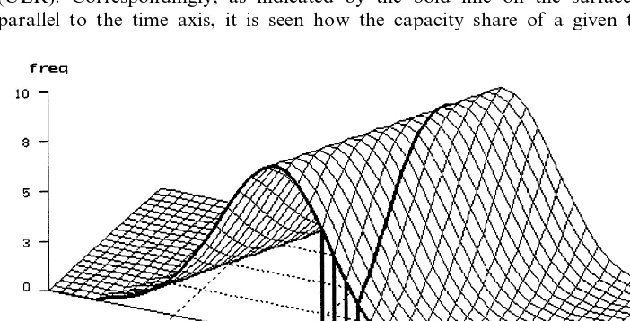
Fig. 1 presents a typical example of the equilibrium evolution of an economy (the underlying numerical details are given in the next section). The diagram clearly shows how the frequency distribution of the techniques’ capacity shares moves regularly over time toward the techniques with lower unit labour requirements (ULR). Correspondingly, as indicated by the bold line on the surface running parallel to the time axis, it is seen how the capacity share of a given technique
Fig. 1. Frequency distributions of techniques on a wave train. Note: Bars indicate frequencies (in %) of techniques with high unit labour requirements (ULR) at timet=20.
8Formally, withN+1=N
t+1=Nt+Tandz=zN−i=z(N+1)−(i+1), the relationship readsf[lnz+
steadily declines in the later stages of its life-cycle. (Its rise in the early stages, when it was still among the most efficient techniques, is hidden by the crest of the distribution surface.) The wave train function f(·) can be read off along the ULR-axis at, for example, t=20.
The unit costs of the active techniques at that date range from a high ofal2=52.7 to a low ofa12+27=12.2 (see the bold line att=20). That is, the new techniques are more than four times as productive as the old vintages. Though the only purpose of Fig. 1 is to illustrate the properties of a highly stylized economic model, these differences in efficiencies might not be too extreme. Thus, to emphasize the economic significance of his general approach, (Iwai, 1984, p. 324) gives a represen-tative example of the frequency distribution of an industry in the USA (the metal stamp industry) where the ratio of payroll to value added covers a range from 0.15 to 0.859
.
Applying the concept of a wave train to system (1 – 11) raises three questions: Does a wave train {k*i (t)} exist? Is it uniquely determined? Is it globally stable? The
latter means that starting from an arbitrary initial frequency distribution {ki(0)},
the resulting solution {ki(t)} of (1 – 11) converges toward the wave train capacity
shares {k*i (t)} as t gets large.
These problems have been subjected to a rigorous mathematical analysis by Henkin and Polterovich (1991) in another, similarly elementary Schumpeterian model. Under a reasonable set of conditions. the authors prove existence and uniqueness of a wave train as well as its global stability. Unfortunately, the (quite elaborated) analysis cannot be readily carried over since the present model differs in a number of specification details. However, existence and the powerful global stability result were fully confirmed in all our numerical simulations. As we have found no reason to harbour any doubts, we do not pursue the mathematical issue any further10.
The property of global stability establishes the economic significance of the long-run equilibrium notion of a wave train. Actually, the global stability was also exploited to compute the wave trains in the numerical investigations below. Accordingly, we initialized the dynamic process (1 – 11) with an arbitrary distribu-tion of capacity shares {ki(0)} att=0, and let it run for so long until Eq. (12) was
approximately satisfied. Then, setting the wage rate back to w=w(0), the process was rerun with the capacity shares just found as the initial frequency distribution. Against the background of the classical theory of income distribution, another feature of interest are the wages and profits on a wave train. Since there is now no longer a uniform rate of profit, we refer to the average profit rate in order to characterize the position of profit receivers by a single number. Denoting by6the share of total wages in gross national income (6=wL/Y), we have
9Of course, these differences cannot be directly compared to that of Fig. 1 since we have no information about the probably varying capital-output ratios in Iwai’s example.
y(t)=w(t)a¯(t) (16)
(cf. the remark on Eq. (7)). Using Eq. (6), the average rate of profit can be written as11
r¯(t)=1−6(t)
b −d=
1−w(t)a¯(t)
b −d. (17)
Since by hypothesis real wages w(t) grow at the same rate at which the unit labour requirements of the BPT decline,w(t)a¯(t) does not systematically rise or fall in the long-run. That is, 6(t+T)=w(t+T)a¯(t+T)=w(t)a¯(t)=6(t) for all t, while between two innovations6(t) may fluctuate on a small scale (these intermedi-ate fluctuations are neglected in the following discussion). By the same token, it is ensured that the average rate of profit remains constant in the course of the process. Hence, if an initial real wage ratew(0) is exogenously given, it has associated with it a wave train solution {k*i (t)} of the evolution of capacity shares, and these in
turn determine the average rate of profitr¯as well as the overall growth rate of the economy,g¯=sr¯. In this sense, the degree of freedom from the classical theory of income distribution is maintained.
On the other hand, also the average rate of profit r¯ may be chosen as the exogenous variable. Observe that, by virtue of Eq. (17), this is tantamount to fixing the wage share6. In the computation of the corresponding wave train, we can then replace Eq. (11) with Eq. (16) and set directlyw(t)=6/a¯(t).
Knowledge of the real wage rate w(0) on a wave train is not yet sufficient to assess the position of workers on this long-run equilibrium growth path; we also have to know the general level of technology at that time, t=0. To discuss variations of income distribution, it is therefore appropriate to deflate the real wage by an index of labour productivity. However, the weights constituting such an index should be independent of the frequency distribution of techniques, which will generally change from one wave train to another. This requirement rules out average productivityq¯=1/a¯as a deflator. Instead, it appears natural to employ the labour productivity of the BPT for this purpose. Looking at wages in the middle between two innovations, define
v=w(T/2)/q–N=w(T/2)aN, whereN=No=NT/2 (18)
It will be clear by now that on a wave train we have w(tm)/q–N(m)=v for all
mIN, where tmmT+T/2, N(m)NmT+T/2. This means that if we study changes in income distribution, we exogenously fix the deflated real wagevand set the initial real wagew(0) such that, on the equilibrium path,w(T/2)=vqN comes
about (N=No). The wave train distribution functionf(·) is subsequently used to
compute the corresponding average rate of profit12 .
11In all what follows it will be understood that averages like r¯, a¯andz¯(the average cost gap) are based on the capacity sharesk*i of a wave train.
Before we illustrate the construction of a wage-profit frontier in this way, we should stress an important conceptual difference from income distribution in the production price systems of the classical theory. In this type of analysis, the study of income distribution, given the ‘book of blueprints’ of techniques, requires the computation of relative prices, while at least in single production systems quantities do not interfere. In the present context of a one-good economy, relative prices are no problem (they would reappear if we tried to set up a two-sectoral version of the model). However, given the path of technical progress, the determination of the distributional variables v and r¯ requires the computation of the equilibrium frequencies of the techniques’ capacity shares. As already indicated in the introductory section, the classical dichotomy between prices and quantities therefore no longer obtains. Despite the highly simplified assumptions on technology, a study of income distribution in an evolutionary economy has to integrate the quantity side right from the outset. It has already been noted above that if, instead of the deflated real wagev, the wage share6is taken as the exogenous variable, the average rate of profit can be directly determined by Eq. (17) without further knowledge of the capacity shares. However, quantities will then interfere as soon as the assumption of a one-good economy is dropped. More importantly, the interdependence between the price and the quantity side under a given wage share occurs, almost trivially, already at a much more elementary level, in basic (multisectoral) production price systems with a uniform rate of profit and best-practice techniques only (cf. Franke, 1998b, 1999). This inconvenience is certainly one of the reasons why classical analysis normally chooses real wages, rather than the wage share, to characterize the position of workers. As we wish to discuss the classical theory within its own preferred setting, we here follow this tradition.
4. Determinants of income distribution
To study the evolution of the economy on a wave train by means of computer simulations, we now have to specify the numerical parameter values. One set of parameters is given by familiar macroeconomic magnitudes: the capital-output ratio
b, the rate of depreciationdand the propensitysto save out of profits. On the basis of Simon (1990), they are fixed as follows,
b=1.70 d=0.0461 d=0.2670 (19)
(again, see the appendix for further details). The other set of parameters governs technological diffusion and innovation: the annual rate of technical progressl, the
innovation timeT(the interval between two innovations), the length of the set-up phaseTu, the autonomous rate of change kat which the capacity share of the BPT increases over this period, and the responsivenessrof investors to differential profits. Here we put13
l=0.029 T=2.00 Tu=0.10 k=0.02 r=1.00 (20)
The innovation parameters T, Tu, and k can be encapsulated in a single parametern defined as
n=kTu/T (21)
The motivation for this definition and its relationship to Iwai’s (1984) stochastic innovation hypothesis is discussed in Franke (1998a). The remarkable point is that (essentially) the same wave train distribution function f(·) is brought about by different combinations ofT,Tuand kthat give rise to identical values ofnin Eq. (21)14.
Finally, we take the deflated real wage rate v as the exogenous variable for income distribution and set
v=0.307 (22)
(Recallv=w(T/2)/qNfrom Eq. (18), withN=No=NT/2). Eqs. (19) and (20) and Eq. (22) may serve as a base scenario. In particular, the special choice ofv=0.307 results in the following values of the wage share, the average profit rate, and the capital growth rate,
6(T)=70.02%, r¯(T)=11.22%, g¯(t)=sr¯(t)=3.00% (23)
which prevail on the wave train in the middle between two innovations, at time
t=T/2. Eq. (23) shows that the model can be calibrated such as to be roughly compatible with empirical values of the macroeconomic key variables here involved. The remainder of the paper is concerned with comparative dynamnics. Accord-ingly, some of the exogenous parameters are varied and the characteristics of the corresponding equilibrium growth paths are studied. In this respect, note first that variations in the exogenous rate of technical progress l have trivial effects on income distribution, since by constructionldetermines directly the growth rate of real wages. In the present setting it is therefore meaningless to compare two economies with different values ofl.
A most important case, however, is a change in the responsivenessrof investors to differential profits. Although r certainly has its institutional foundations, it is also of a psychological nature. Given the economy’s institutions,rmay be regarded as a psychological coefficient. Now, it is a centrepiece of the classical theory that the long-run equilibrium position is independent of such a reaction intensity. In this theory, the only significance ofrwould be in the disequilibrium adjustment process toward the steady state. For example, a mathematical analysis of a gravitation process might reveal that this parameter must not be too large if stability is to be ensured. By contrast, in the present Schumpeterian framework it turns out that the
14For example, an increase inTtogether with the corresponding reduction ofkorT
responsiveness r already has a bearing on the long-run equilibrium itself. For example, maintain the other parameter values in (19, 20, 22) and increase the responsiveness to, say,r=1.20. Income distribution and growth on the new wave train are then given by
6(T)=66.31%, r¯(T)=13.40%, g¯(t)=3.58% (t=T/2) (24)
Comparing these values with Eq. (23), it is seen that a higher responsiveness of investors, or intensified competition, improves the position of profit earners and also leads to faster growth if workers receive the same real wages.
The qualitative changes in the wage share 6 and the average profit rate r¯ are easily explained. A higher responsivenessrmeans that the more efficient techniques expand more rapidly than before. Average labour productivityq¯is therefore higher, which is tantamount to a lower average cost gapz¯=a¯/aN=1/(q¯aN) (cf. Eq. (8) and
Eq. (14)). Recalling Eq. (16) and Eq. (18) and using wa¯=(w/qN)(a¯/aN)=vz¯, it
remains to note that the wage share is related to the average cost gap by
6=vz¯. (25)
In the presence of unchanged deflated real wages we therefore have that faster diffusion, which reduces the average cost gap z¯, yields a lower wage share and a higher average rate of profit. Again we emphasize that this result and the underly-ing mechanism have no counterpart in the classical theory of distribution and growth.
In the further discussion of the long-run equilibria it will be useful to refer to the original Iwai (1984) model. Iwai characterizes the techniquesi by their unit costsi
and postulates that the motions of the capacity shares are directly governed by these unit costs:
k:i= −g(lnci−lnci)ki (26)
where gis a constant parameter that measures the general speed of technological diffusion (Iwai, 1984, p. 328). In Franke (1998a) the intuition is confirmed that a higher value ofgindeed reduces the cost gap (analogously defined) on a wave train of this economy15. This result is central to the following discussion of the compar-ative dynamics.
Now, the profit rate differentials in the present model can be expressed as
ri−r¯=(−6/b)(ai−a¯)/a¯. With Eq. (25), the upper part of the diffusion Eq. (10)
can thus be rewritten as
k:i=
−rvz¯ b
ai−a¯
a¯ ki (27)
As the percentage deviations of unit labour requirementsai in (27) correspond to
Iwai’s log differences in unit costs ci in (26), we have the following approximate
relationship between the concept of the technological speed of diffusion and some central parameters in our model,
g:g%rvz¯ b =
r6
b (28)
Let us also callg% the speed of technological diffusion.
Before going on, it is worth mentioning that, had the investment function (9) been specified as
gi=s[r¯+r(ri−r¯)] (9a)
Eq. (28) would becomeg:srvz¯/b. In this case, income distribution on the wave trains would also be dependent on the propensity to save out of profits, another result which is alien to the production price systems of the classical theory. Evidently, an increase in s has then the same effect as an increase in r. Hence, under Eq. (9a) a higher savings propensity would lead to a lower wage share and a higher average rate of profit. It is also worth mentioning that the growth rateg¯
of the economy would rise more than proportionately.
While in Iwai’s model the speed of diffusion is an exogenous parameter, Eq. (28) reveals that it is endogenous in our setting if the real wage ratevis chosen as the exogenous income distribution variable16. Nevertheless, despite the interference of the average cost gap z¯ a ceteris paribus increase in the responsiveness r to profit rate differentials will also cause the general speed of technological diffusion g% to rise. Although, as indicated above, the average cost gap z¯ decreases, the direct influence ofrremains dominant, so that the productrz¯in (28) increases. (In fact, if rz¯ were to decrease, the lower value of g%, according to the remark on Eq. (26), would be associated with a higher value of z¯, which would be a contradiction).
This line of reasoning can be readily carried over toceteris paribuschanges in the deflated real wage rate v. Just like r, a rise in v speeds up the diffusion of new techniques and thus lowers the average cost gap z¯, but again not so much as to diminishg% in Eq. (28). Since by (25) the higher productvz¯means a higher share of wages6, we can conclude that an increase in real wages v induces a fall of the average rate of profitr¯in the new long-run equilibrium. In this sense, the classical inverse relationship between real wages and profits is re-established.
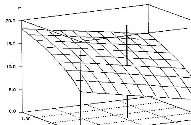
The income distribution effects just discussed are summarized in Fig. 2, which shows the response surface of the average rate of profit r¯ on the respective wave trains under variations of the deflated real wage rate v and the responsiveness coefficientr. Over the range of parameters considered, the relationship between r¯
and v is nearly linear. On the other hand, r¯ is a convex function of r, i.e. the increments in the profit rate induced by a further rise in r become smaller with higher values ofr.
Fig. 2. Average rate profit (r¯) on a wave train under variations of the deflated real wage rate (v) and the responsiveness of investors (r). Note: the reference stick indicates the base scenario.
Having discussed the effects ofvandr, the parameternof Eq. (21) above, which characterizes the introduction of new techniques, should not be neglected. Since a rise in n corresponds to a faster diffusion of the best-practice techniques in their set-up phase, the effect will be expected to be similar to an increase inr. This is certainly true as regards the average profit rate or the wage share. To give an example, raisingnin the base scenario from n=0.0010 to n=0.0030 increases the average profit rate by about 4%, while reducingnton=0.0003 lowersr¯by almost 4% (vis-a-visr¯=11.22% andn=70.02% in the base scenario, the precise figures are
r¯=15.23% and 6=63.21% in the first case, and r¯=7.32%, 6=76.66% in the second case).
However, it should also be noted that a change innaffects the general speed of
technological diffusiong% as it was specified in Eq. (28). The decrease of the cost gapz¯that is associated with a rise ofnmeans. perhaps some what surprisingly. that a faster introduction of new techniques reduces the overall speed of diffusion g%. While g%=0.412 in the base scenario, we obtain, g%=0.372 for n=0.0030 and
g%=0.451 forn=0.00317.
5. A note on the law of the falling rate of profit
In this section we return to the remaining magnitudeb in the specification of the speed of diffusiong%in (28) that has not been varied yet. Formally, a higher capital output ratiob has the same effect as a ceteris paribusdecrease in r: it raises the average cost gapz¯on the new wave train distribution. The corresponding average rate of profit therefore declines for two reasons: one is the direct effect of the higher denominatorbin the definition of profit rates, the other is the indirect effect of the change in the wage share, which owing to Eq. (25) is driven up by the rise inz¯18. The result is reminiscent of the Marxian law of the falling rate of profit that is attributed to a rising trend in the organic composition of capital. In the Sraffian production price systems, this subject is usually studied in the form of capital-using and labour-saving technical change. It is, however, well-known that here Okishio’s theorem holds (Okishio, 1961). When a new method of production replaces an existing one because of higher profitability in a given system of production prices, then, if the real wage remains fixed, the uniform rate of profit in the new equilibrium system will inexorably exceed the original profit rate. There is no scope for a falling rate of profit in this setting. While Okishio’s theorem highlights the salient point in the discussion on the internal consistency of the Marxian law, that capitalists would avoid any technical change that reduces the profit rate, the problem of coming to terms with ‘micro-rational’ behaviour is resolved in the present evolutionary framework. At any point in time, the innovation that yields the highest rate of profit will be introduced, irrespective of the kind of technical change it involves. Clearly, an investor who hesitates to invest in such a technique with a higher capital-output ratio because he is afraid of the consequences for the average profit rate in later years, even if he were able to foresee them, would only earn less profits than his competitors. And of course, the a6eragerate of profit is not his concern19.
In the above experiment where two economies with the same growth path of labour productivity but different capital-output ratios b are compared, there are two magnitudes that affect the organic composition of capital,x. In Marxian terms,
x is the ratio of constant capital to variable capital. Translating this as the capital – wages ratio and decomposing it asx=(K/wL)=(K/Y) (Y/wL)=b/6=b/
vz¯, it is seen that the higher average cost gap z¯in the second economy with the
18We may note in passing an interesting phenomenon that occurs if alternatively the wage share6is the distributional variable that is held constant. Then not only does the average profit rate decline by Eq. (17), but, sincez¯rises again, also the deflated real wage ratev=6/z¯. Incidentally, this cannot possibly happen in a production price framework where, in the presence of a fixed wage share, an increase in some coefficients of the capital stock matrix B decreases the (uniform) rate of profit, but raises the real wage rate; cf. Fig. 1 in Franke (1999).
higher value ofbhas a negative impact onx. Nevertheless, the positive effect from
b is dominant, so that indeed the organic composition of capital turns out to be higher in the second economy. (The argument is the same as in the previous section forr: a higher b reducesg%=rvz¯/b in (28), despite the rise in z¯, so that x=b/vz¯
increases).
On the other hand, the result that the economy with the higher capital-output ratio exhibits a lower average rate of profit is not particularly exciting. Since labour productivity was assumed to grow at the same rate in this economy, the gains in profitability accruing to an innovation are less than in the economy with the lower value of b, i.e. the differences rN−rN−1, and generally ri−ri−1, are smaller. It therefore comes as no surprise that also the average rate of profit is bound to fall. The discussion so far was based on theceteris paribusassumption of a fixed value of the responsiveness to differential profits, r. This concept may be considered to be too mechanistic. The lower differencesri−ri−1 in Eq. (10) imply that investors in the profitable techniques wish to expand their market shares less rapidly. By contrast, another basis of comparing two economies with different capital-output ratios may be that one fixes the differences (k:i/ki)−(k:i−1/ki−1) in the growth rates of two successive techniquesiandi−1 at which they increase their market shares. This hypothesis is captured by variations of r proportionally to b. In fact, if the ratio r/b remains unaltered in the speed of technological diffusion g% in (28), the average cost gap z¯on the wave train would not be affected either. Since the unit labour requirements ai are identical, Eq. (27) shows that in both economies the
market shares of the techniques evolve in the same way. Even if the alternative basis of comparison may be felt to be somewhat arbitrary, the few observations may suffice to indicate that a careful investigation into the effects of capital-using technical change has to include more aspects than just the changes of the capital-output ratio in some definitional relationships20
.
Note also that if, over longer periods, capital-using technical change is associated withhighergrowth rates of labour productivity while wages continue to increase at the original growth rate, the wage share would systematically fall and (possibly besides unemployment) the economy would sooner or later run into serious conflicts over income distribution. This is only one point where it becomes clear that, if we go beyond the narrow constraints of the present equilibrium setting, the analysis needs to be complemented by a study of additional dynamic mechanisms.
6. Conclusion
The model studied in this paper is an elementary extension of an evolutionary process advanced by Iwai (1984). Translating the Schumpeterian ideas on the dynamic interaction of technological diffusion and innovation into a formal
guage, Iwai’s main goal was to question the appropriateness of the classical and neoclassical concept of long-run equilibrium. He demonstrated that an economy’s state of technology will indeed be in a perpetual disequilibrium (from the viewpoint of classical and neoclassical model building). Although the evolutionary pressure on profit-seeking firms constitutes a mechanism that steers the economy toward a classical (or neoclassical) equilibrium in which all firms use the most efficient production method available, the function of innovation lies precisely in upsetting this equilibrating tendency. In the long-run, the opposite forces of diffusion and innovation balance, which implies that a multitude of diverse production methods with a wide range of efficiencies will coexist forever.
This general idea comes most clearly to the fore in a deterministic setting where innovations occur at regular intervals everyT years. (Iwai’s original hypothesis of stochastic innovations would have complicated our analysis.) While production methods come into existence, run through a life-cycle and eventually die out, the whole spectrum of different techniques reproduces itself, only at an ever increasing scale as time progresses. This means that the role of techniquei at some timet is taken over by its more advanced successor at a later point in time,t+T. Drawing on Henkin and Polterovich (1991), this smooth evolution of the economy has been called a wave train. Compared to the usual (neo-)classical conception, it may be said that wave trains provide a notion of long-run equilibrium at a higher level. On the other hand, the balanced growth paths here examined should not be taken too literally. Although they are attractors and, once perturbed, the economy finds back to them, the adjustment process would take a long span of time; typically several decades as shown in Franke (1998a). There are several parameters in the model that one could not reasonably consider to remain fixed over these periods. So we see our paper’s main contribution, not so much in providing an elaborate equilibrium analysis, but in widening the narrow classical and neoclassical perspective on technical progress. Correspondingly, the main purpose of a highly stylized model such as the present one is to serve as a frame of reference.
endogenous technical change (which might also fail to be Harrod-neutral), then this type of comparison will have to be replaced with a comparison of the growth rates of real wages, or with a comparison of the wage shares in national income.
Acknowledgements
Insightful comments by two anonymous referees are gratefully acknowledged.
Appendix A
Generally in the simulations, time is sliced into (arbitrarily) small economic adjustment periods of lengthh and the discrete-time analogues with step size h of the differential equations are used. This device. while simpler than the Runge – Kutta approximations, is not purely technical but has an obvious economic interpretation.
Thus, in ‘normal’ periods wheretQU(Nt), we take the capital growth rates of Eq.
(9) and determinek0i(t+h)=ki(t)+h [sr¯(t)+r(ri(t)−r¯(t))]ki(t) for i5Nt, which
corresponds to the le6el of capital stocks in the next period t+h. Subsequent renormalization yields the (capital and) capacity shares, ki(t+h)=k0i(t+h)/j5N k0i(t+h).
The second part of Eq. (10), which concerns the set-up phase tU(Nt), is a
shorthand notation for the following procedure. The growth rates of the capital stocks for techniquesi5Nt−1 are resealed such that the growth rate of the total
capital stock continues to be equal tosr¯. That is, definingg˜i=sr¯(t)+r(ri(t)−r¯(t))
anda=(sr¯−k)/j5N−1g˜jkj(t), the growth ratesgifor i5Nt−1 are determined by
gi(t)=ag˜i
21. For the BPT we put
kN(t+h)=kN(t)+hkby way of Eq. (5), whereas
for the ordinary techniques i5Nt−1 we first compute k0i(t+h)=ki(t)+ h gi(t)ki(t) and thenki(t+h)=k0i(t+h)/[kN(t+h)+j5N−1k0i(t+h)].
Another detail are the old vintages, which tend to disappear in the long-run. For practical reasons we reset the capacity share of the least productive technique back to zero in the computer simulations when it declines below a benchmark of 0.1%. To derive Eq. (15) note that for a best-practice technique N=NmT one has lnaN+gwmT=lnaN+gwmT=lnaNoªC. Thus, with t=mT+t, ln ai+gwt= (ln ai−lnaN)+lnaN+gwt=ln(ai/aN)+lnaN+gwmT+gwt=lnzN−i+gwt+C, and Eq. (15) follows from Eq. (13).
The numerical parameters in Eq. (19) are obtained as follows. The capital-output ratio is taken directly from Simon (1990, p. 151). Next, in obvious notation, the ratio of gross investment to GNP is equal to (K: +dK)/Y=g¯b+db. Adopting Simon’s (p. 153) ratio of 16% and setting g¯=3% yields the value ofd. As for the savings propensity s. we take a wage share6=70% (cf. Simon, p. 150), compute the
profit rate r¯=(1−6)/b−d, and thus retrieve s from the Cambridge equation as
s=g¯/r¯.
References
Franke, R., 1998. Wave trains and long waves: a reconsideration of Professor Iwais Schumpeterian dynamics, forthcoming. In: Delli Gatti, D., Gallegati, M., Kirman, A. (Eds.), Market Structure, Aggregation and Heterogeneity. Springer, Berlin.
Franke, R., 1998. Quantities and prices. In: Kurz, H.-D., Salvadori, N. (Eds.), The Elgar Companion to Classical Economics; L – Z. Edward Elgar, Cheltenham, pp. 236 – 238.
Franke, R., 1999. Technical change and a falling wage share if profits are maintained. Metroeconomica 50, 35 – 53.
Henkin, G.M., Polterovich, V.M., 1991. Schumpeterian dynamics as a non-linear wave theory. J. Math. Econ. 20, 551 – 590.
Iwai, K., 1984. Schumpeterian dynamics, part II: Technological progress, firm growth and economic selection. J. Econ. Behav. Organization 5, 321 – 351.
Metcalfe, J.S., 1997. Evolutionary Economics and Creative Destruction. Routledge, London (Quotation from manuscript, February, 1997).
Okishio, N., 1961. Technical change and the rate of profit. Kobe University Econ. Rev. 7, 86 – 99. Schumpeter, J.A., 1950. Capitalism, Socialism and Democracy. Harper and Row, New York. Silverberg, G., Lehnert, D., 1993. Long waves and evolutionary chaos in a simple Schumpeterian model
of embodied technical change. Structural Change Econ. Dynamics 4, 9 – 37.
Silverberg, G., Verspagen B., 1997. Of artificial and real worlds, or from modeling to econometric metaphor. Maastricht Economic Research Institute on Innovation and Technology, Mimeo. Simon, J.L., 1990. Great and almost-great magnitudes in economics. J. Econ. Perspect. 4, 149 – 156. Soete, L., Turner, R., 1984. Technology diffusion and the rate of technical change. Econ. J. 94, 612 – 623.