www.elsevier.com/locate/spa
On stationary solutions of delay dierential equations
driven by a Levy process
Alexander A. Gushchin
a, Uwe Kuchler
b;∗aSteklov Mathematical Institute, Gubkina 8, 117966 Moscow GSP-1, Russia
bInstitut fur Mathematik, Humboldt-Universitat zu Berlin, Unter den Linden 6,
D-10099 Berlin, Germany
Received 24 March 1999; received in revised form 4 October 1999; accepted 22 December 1999
Abstract
The stochastic delay dierential equation
dX(t) = Z
[−r;0]
X(t+u)a(du) dt+ dZ(t); t¿0
is considered, whereZ(t) is a process with independent stationary increments and ais a nite signed measure. We obtain necessary and sucient conditions for the existence of a stationary solution to this equation in terms of aand the Levy measure of Z. c 2000 Elsevier Science B.V. All rights reserved.
Keywords:Levy processes; Processes of Ornstein–Uhlenbeck type; Stationary solution; Stochastic delay dierential equations
1. Introduction
Leta be a nite signed measure on a nite interval J= [−r;0]; r¿0. Consider the equation
X(t) =
X(0) +
Z t
0
Z
J
X(s+u)a(du) ds+Z(t); t¿0;
X0(t); t∈J:
(1.1)
Here Z= (Z(t); t¿0) is a real-valued process with independent stationary increments starting from 0 and having cadlag trajectories, i.e. Z is a Levy process, and X0=
(X0(t); t ∈ J) is an initial process with cadlag trajectories, independent of Z. The
question treated in this note concerns the existence of stationary solutions to (1.1). If r= 0, the answer to this question is known. The equation
X(t) =X(0) +
Z t
0
X(s) ds+Z(t); t¿0 (1.2)
∗Corresponding author.
(X(0) and Z are independent) admits a stationary solution if and only if
¡0 (1.3)
and
Z
|y|¿1
log|y|F(dy)¡∞; (1.4)
where F denotes the Levy measure of Z. This stationary solution X is called a sta-tionary process of Ornstein–Uhlenbeck type. Its distribution is uniquely determined by and the Levy–Khintchine characteristics of Z, in particular, the law of X(t) is the distribution of
U=
Z ∞
0
etdZ(t):
Essentially, these results are due to Wolfe (1982). Their multi-dimensional versions were considered, in particular, by Jurek and Vervaat (1983), Jurek (1982), Sato and Yamazato (1983), Zabczyk (1983) and Chojnowska-Michalik (1987).
In this paper we show that a stationary solution of (1.1) exists if and only if the equation
h() :=− Z
J
eua(du) = 0 (1.5)
has no complex solutions with Re¿0, and condition (1.4) holds. Thus, in com-parison with the Ornstein–Uhlenbeck case, condition (1.3) is replaced by
{∈C|h() = 0; Re¿0}=∅: (1.6)
The distribution of a stationary solutionX is unique for givena and the characteristics of Z, and the law ofX(t) is the distribution of
U=
Z ∞
0
x0(t) dZ(t); (1.7)
wherex0(t) is the so-called fundamental solution of the corresponding (1.1)
determin-istic homogeneous equation (see the denition in Section 2). IfZ is a Wiener process and a is concentrated in points 0 and r, these results were proved by Kuchler and Mensch (1992).
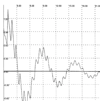
As in the case of Eq. (1.2), a stationary solution of (1.1) exists if and only if the integral in (1.7) converges in an appropriate sense. But, unlike the Ornstein–Uhlenbeck case (where x0(t) = et), the fundamental solution x0(t) is not necessarily a positive
monotone function, for example, it may oscillate around 0 under (1.6), see Fig. 1. Thus, the proof of the necessity of (1.6) and (1.4) for the convergence of the integral in (1.7) is not so straightforward as in the case r= 0.
Stochastic dierential equations of type (1.1) can be considered as linear stochastic dierential equations in some Hilbert spaceH:
dXt=AXtdt+ dZt; t¿0; (1.8)
where A is the innitesimal generator of a strongly continuous semigroup (Tt)t¿0 of
Fig. 1. The fundamental solutionx0(t) fora(du) =−0(du) + 0:7−0:2(du)−0:3−0:4(du)−0:2−0:6(du) +
5:5−0:8(du)−5:4−1(du).
Da Prato and Zabczyk (1992) for details. Chojnowska-Michalik (1987) studied the problem of the existence of stationary distributions for the solutions of (1.8) and ob-tained the suciency of conditions similar to (1.6) and (1.4). Under an additional assumption on the semigroup (Tt)t¿0 ((Tt) can be extended to a group on R), which
is not satised in our case, she proved also the necessity of these conditions.
The assumption that the initial processX0 andZ are independent is important for the
above result. Otherwise, (1.6) is not necessary for the existence of a stationary solution, cf. Theorem 3.1 in Jacod (1985) and Theorem 20 in Mohammed and Scheutzow (1990).
2. Preliminaries
2.1. Deterministic delay dierential equations
Since Eq. (1.1) involves no stochastic integrals and is treated pathwise, we will formulate a number of results for solutions of Eq. (1.1) with deterministic Z and X0, for which we refer to Hale and Verduyn Lunel (1993), Diekmann et al. (1995),
Myschkis (1972), and also to Mohammed and Scheutzow (1990).
A real-valued functionX(t); t¿−r, is called a solution of the equation (1.1), if it is locally integrable and satises (1.1) for all t¿−r or only for t¿0 if the initial condition is not specied (here and below “integrable” means “integrable with respect to the Lebesgue measure”; the double integral in (1.1) exists for such functions by the Fubini theorem).
Assume that a nite signed measureaon J, a real-valued locally integrable function Z on R+ satisfying Z(0) = 0, and a real-valued integrable function X0 on J are given
(only sucha; Z, and X0 will be considered in the sequel). Then Eq. (1.1) has a unique
solution. This solution is cadlag (resp. continuous, resp. absolutely continuous) onR+
if and only if Z is cadlag (resp. continuous, resp. absolutely continuous).
Given a measure a, we call a function x0: [−r;∞[→R the fundamental solution
of the homogeneous equation
X(t) =
X(0) +
Z t
0
Z
J
X(s+u)a(du) ds; t¿0;
X0(t); t∈J;
(2.1)
if it is the solution of (2.1) corresponding to the initial condition
X0(t) =
(
1; t= 0; 0; −r6t ¡0:
In other words, a function x0(t); t¿−r, is the fundamental solution of (2.1) if it is
absolutely continuous on R+; x0(t) = 0 for t ¡0; x0(0) = 1, and
˙ x0(t) =
Z
J
x0(t+u)a(du) (2.2)
for Lebesgue-almost allt ¿0. To facilitate some notation in the sequel it is convenient to put x0(t) = 0 for t ¡−r.
The solution of (1.1) can be represented via the fundamental solution x0 of (2.1):
X(t) =
x0(t)X0(0) +
Z
J
Z 0
u
X0(s)x0(t+u−s) ds a(du)
+
Z
[0; t]
Z(t−s) dx0(s); t¿0;
X0(t); t∈J:
(2.3)
Remark. The domain of integration in the last integral in (2.3) includes zero:
Z
[0; t]
Z(t−s) dx0(s) =Z(t) +
Z
]0; t]
The asymptotic behaviour of solutions of Eqs. (1.1) and (2.1) fort→ ∞ is connected with the set of complex solutions of the so-called characteristic equation
h() = 0; (2.4)
where the function h(·) is dened in (1.5). Note that a complex number solves (2.4) if and only if (et; t¿−r) solves (2.1) for the initial condition X
0(t) = et; t∈J.
The set :={∈C|h() = 0}is not empty; moreover, it is innite except the case
where a is concentrated at 0. Since h(·) is an entire function, consists of isolated points only. It is easy to check that n ∈ and |n| → ∞ imply Ren → −∞, thus
the set {∈|Re¿c} is nite for every c∈R. In particular,
v0:= max{Re|∈}¡∞ (2.5)
holds. Dene
vi+1:= max{Re|∈; Re ¡ vi}; i¿0:
For ∈denote by m() the multiplicity of as a solution of (2.4).
It is easy to check from (2.2) that 1=h() is the Laplace transform of (x0(t); t¿0)
at least if Re is large enough. (In fact,
1=h() =
Z ∞
0
e−tx0(t) dt
if Re ¿ v0.) Applying a standard method based on the inverse Laplace transform
and Cauchy’s residue theorem, we come to the following lemma which is essentially known and can be found in a slightly dierent form in Hale and Verduyn Lunel (1993) and Diekmann et al. (1995). The proof will be sketched in Section 4.
Lemma 2.1. For any c∈R we have
x0(t) =
X
i:vi¿c
X
∈ =vi
p(t)evit+
X
∈ Re=vi
Im¿0
{q(t) cos(tIm) +r(t) sin(tIm)}evit
+ o(ect);
t → ∞; where p(t) is a real-valued polynomial in t of degree m()−1; q(t) and
r(t) are real-valued polynomials in t of degree less than or equal to m()−1; and
the degree of either q(t) or r(t) is equal to m()−1.
This lemma and the following corollary describe properties of the fundamental solution x0(t), which are crucial for the proof of our main result.
Corollary 2.2. For some ¿0;
lim inf
t→∞
1 t
Z t
0
2.2. Levy processes
LetZ=(Z(t); t¿0) be a Levy process. Throughout the paper a continuous truncation function g is xed, i.e. g:R → R is a bounded continuous function with compact
support satisfying g(y) =y in a neighbourhood of 0.
It is well known, see e.g. Jacod and Shiryaev (1987), that the distribution of Z is completely characterized by a triple (b; c; F) of the Levy–Khintchine characteris-tics, namely, a number b∈R(the drift), a nonnegative number c∈R+ (the variance
of the Gaussian part), and a nonnegative -nite measure F on R that satises F({0}) = 0 and
Z R
(y2∧1)F(dy)¡∞ (2.6)
(the Levy measure of jumps). In particular,
Eexp{iu(Z(t)−Z(s))}= exp{(t−s) b; c; F(u)}; u∈R; s ¡ t;
where
b; c; F(u) := iub−
1 2u
2c+Z
R
(eiuy−1−iug(y))F(dy): (2.7)
Moreover, this triple (b; c; F) is unique, and, for every triple (b; c; F) satisfying the above assumptions, there is a Levy process Z with the characteristics (b; c; F).
In the following, we shall deal with integrals of the form
If(t) :=
Z t
0
f(s) dZ(s);
wheref:R+→Ris a cadlag function of locally bounded variation. In this simple case there is no need to use an advanced theory of stochastic integration (however, let us mention that the results stated below are valid for at least locally bounded measurable f). Indeed, the integral If(t) can be dened by formal integration by parts:
If(t) =f(t)Z(t)−
Z
]0; t]
Z(s−) df(s); (2.8)
where Z(s−) = lims′↑sZ(s′). Of course, this pathwise denition is equivalent to the
usual denitions of stochastic integrals.
The next lemma is a simple exercise. The rst equality in its statement can be found e.g. in Lukacs (1969).
Lemma 2.3. The integral It(f) has an innitely divisible distribution:
Eexp{iuIf(t)}= exp
Z t
0
b; c; F(uf(s)) ds
= exp{ B(t); C(t); F(t)(u)};
where
B(t) :=b
Z t
0
f(s) ds+
Z R
Z t
0
{g(yf(s))−f(s)g(y)}ds F(dy); (2.9)
C(t) :=c
Z t
0
F(t;{0}) = 0;
for any nonnegative measurable function satisfying (0) = 0.
Lemma 2.4. If(t) converges in distribution ast→ ∞if and only if there exist nite
for any nonnegative measurable function.
Remark. The assumptions of Lemma 2.4 do not imply the integrability of b; c; F(uf(s))
on [0;∞[. Of course, if the Lebesgue integral R∞
3. The main result
In this section we assume that there are a xed nite signed measurea onJ and a triple (b; c; F) of the Levy–Khintchine characteristics such that either c ¿0 or F 6= 0. We say that a processX= (X(t); t¿−r) is a solution to Eq. (1.1) if there are a Levy processZ= (Z(t); t¿0) with the characteristics (b; c; F) and a processX0= (X0(t); t∈
J) with cadlag trajectories such that (1.1) holds; moreover Z and X0 are assumed to
be independent. In other words, a cadlag stochastic process X = (X(t); t¿−r) is a solution to (1.1) if
(1) Z(t) =X(t)−X(0)−Rt
0
R
JX(s+u)a(du) ds, t¿0, is a Levy process with the
characteristics (b; c; F);
(2) the processes X = (X(t); t∈J) and Z= (Z(t); t¿0) are independent.
We say that a solution X = (X(t); t¿−r) is a stationary solution to (1.1) if
(X(tk); k6n)= (d X(t+tk); k6n) (3.1)
for all t ¿0, n¿1, t1; : : : ; tn¿−r.
Theorem 3.1. There is equivalence between:
(i) Eq. (1:1) admits a stationary solution;
(ii) there is a solution X of (1:1)such that X(t) has a limit distribution as t→ ∞; (iii) for any solution X of (1:1); X(t) has a limit distribution as t→ ∞;
(iv) v0¡0 and
R
|y|¿1log|y|F(dy)¡∞.
Moreover; in that case for an arbitrary solution X(t) of (1:1)
(v) the distribution of (X(t+tk); k6n);where n¿1; 06t1¡ t2¡· · ·¡ tn are xed;
weakly converges as t→ ∞ to the distribution of the vector Z ∞
tn−tk
x0(s+tk−tn) dZ(s); k6n
; (3.2)
where Z= (Z(s); s¿0)is a Levy process with the characteristics (b; c; F); (vi) the distribution of the process (X(t+s); s¿0) weakly converges in the
Sko-rokhod topology as t → ∞ to the distribution of a stationary solution (Y(s); s¿0); which is uniquely determined due to(v).
Remark. (1) The integrals in (3.2) are dened in Lemma 2.4. The correctness of their denition will be shown in Lemma 4.3.
(2) It follows from the proof of Theorem 3.1 that, given a Levy process Z with the characteristics (b; c; F) on a probability space (;F; P), one can construct, under the condition (iv), a stationary solution on the same probability space if it is large enough, in particular, if there is another Levy process on (;F; P) with the same characteristics independent of Z.
4. Proofs
Proof of Lemma 2.1. According to Lemma I.5.1 and Theorem I.5.4 in Diekmann et al. (1995),
x0(t) =
X
∈ Re¿c
Res
z=
ezt
h(z)+ o(e
ct); t→ ∞: (4.1)
Let ∈ , Re¿c, and m:=m(). Write Laurent’s series of 1=h(z) at z= in the form
1=h(z) =
∞
X
k=−m
Ak()(z−)k; A−m()6= 0:
Since
ezt= et
∞
X
k=0
tk
k!(z−)
k;
the multiplication of the above series yields
Res
z=
ezt h(z)= e
t −1
X
k=−m
Ak()
(−1−k)!t
−1−k
Note that h( z) =h(z) (where a bar means the complex conjugate). Therefore, we have ∈ if and only if ∈ . Moreover, it holds Ak() =Ak( ). Hence, if Im= 0,
then Ak() ∈ R and p(t) =P−1k=−m [Ak()=(−1−k)!]t−1−k. If Im 6= 0, we join
two terms in (4.1) corresponding to and . After simple calculations we obtain (for deniteness, we assume that Im ¿0)
Res
Proof of Corollary 2.2. According to Lemma 2.1, it is enough to check that, for some ¿0,
for a continuous function f(t) satisfying
Proof of Lemma 2.4. According to the well-known conditions for the weak con-vergence of innitely divisible distributions (see e.g. Remark VII.2.10 in Jacod and Shiryaev, 1987), If(t) converges in distribution as t → ∞ if and only if there is a
nite limit limt→∞B(t) and the measures C(t)0(dy) + (y2∧1)F(t; dy) weakly
con-verge to a measure ˜C0(dy) + (y2∧1) ˜F(dy) with ˜F({0}) = 0, the limit distribution
being innitely divisible with the characteristics (B(∞);C;˜ F˜) (here0(·) is the Dirac
measure at 0). In our case F(t)−F(s) is a nonnegative measure for all t ¿ s due to (2.11). Therefore, the conditions just mentioned take place if and only if the condi-tions of the lemma are satised; moreover, ˜C=C(∞) and ˜F=F(∞). It remains to note thatIf(t) is a cadlag process with independent increments, hence the convergence
in distribution of If(t) as t → ∞ implies the convergence of If(t) almost surely as
t→ ∞.
Before proving Theorem 3.1 we need a number of preliminary lemmas. We keep the notation and the conventions of Section 2.
Lemma 4.1. Assume that v0¡0 and X(t) is a solution of(deterministic) Eq. (2:1).
Then limt→∞X(t) = 0.
Proof. According to (2.3),
X(t) =x0(t)X0(0) +
Z
J
Z 0
u
X0(s)x0(t+u−s) ds a(du); t¿0:
By Lemma 2.1,|x0(t)|6ce−t,t¿0, for somec ¿0 andsuch that 0¡ ¡|v0|, from
which the claim follows easily.
Lemma 4.2. Let z: [0; T]→R; T¿0; be a cadlag function. Put
X(t) =x0(t+T)z(T)−
Z
]0;T]
z(s−) dx0(t+s); t¿−r: (4.2)
Then (X(t); t¿−r) is a cadlag solution of the homogeneous equation (2:1).
Remark. If z has a bounded variation and we put z(t) = 0 for t ¡0, integration by parts gives
X(t) =
Z
[0;T]
x0(t+s) dz(s); t¿−r;
i.e. X(·) is a mixture of x0(·+s), s∈[0; T]. Thus, the statement of the lemma is not
surprising since every x0(·+s) is a solution of (2.1).
Proof. If z is a piecewise constant function, the claim follows immediately from the previous remark. For the general case, use a uniform approximation ofz by piecewise constant functions.
Lemma 4.3. Let f:R+ → R be a function of locally bounded variation such that
|f(t)|6ce−t for some c ¿0 and ¿0. If(1:4) holds; then If(t) has a limit
Proof. We will check the conditions of Lemma 2.4. First, in view of (2.10),
Let us show that
sup
The right-hand side of the previous inequality is nite in view of (2.6) and (1.4). In view of (2.9), in order to show that
B(t)→b
it is enough to check that
Now (4.6) follows from (4.7), (4.8), (2.6), and (1.4), and the statement follows from (4.3) – (4.5) and Lemma 2.4.
Lemma 4.4. Let f:R+→R be a locally bounded measurable function such that
Z R
Z ∞
0
(y2f2(s)∧1) ds F(dy)¡∞
and
lim inf
t→∞
1 t
Z t
0
1(|f(s)|¿e−s) ds ¿0
for some ¿0 and ¿0. Then (1:4) holds.
Proof. Put
G(t) =
Z t
0
1(|f(s)|¿e−s) ds:
By the assumption, there are a T ¿0 and an ¿0 such that G(t)¿t for all t¿T. We have
Z R
Z ∞
0
(y2f2(s)∧1) ds F(dy)
¿
Z
|y|¿−1eT
Z −1log(|y|)
0
(y2f2(s)∧1)1(|f(s)|¿e−s) ds F(dy)
=
Z
|y|¿−1eT
G(−1log(|y|))F(dy)
¿−1
Z
|y|¿−1eT
log(|y|))F(dy):
The left-hand side of the above inequality is nite by the assumptions, so we easily obtain (1.4).
Proof of Theorem 3.1. Let us rst note that by (2.8),
Z
[0; t]
Z(t−s) dx0(s) =
Z t
0
x0(t−s) dZ(s):
Thus, using (2.3), any solution of Eq. (1.1) can be written in the form
X(t) =x0(t)X0(0) +
Z
J
Z 0
u
X0(s)x0(t+u−s) ds a(du)
+
Z t
0
x0(t−s) dZ(s); t¿0: (4.9)
Note also that, by Lemma 2.3,
Z t
0
x0(t−s) dZ(s) d
=
Z t
0
x0(s) dZ(s): (4.10)
Let us prove (iv)⇒(i). LetZ=(Z(t); t¿0) and ˜Z=( ˜Z(t); t¿0) be two independent Levy processes with the same characteristics (b; c; F). To make the idea more clear, let us dene a two-sided Levy process (Z(t); t∈R) by
Therefore, the process X is stationary in the sense of (3.1). Note also that by Lemma 2.4 the characteristic function of vector (3.2) coincides with the right-hand side of (4.12).
We shall show that there exists a modication ofX(t) being cadlag and solving Eq. (1.1). To this aim we shall construct a sequence (XN(t); t¿−r) of cadlag solutions
to (1.1) such that XN(t) converges uniformly in t¿−r as N → ∞almost surely and
lim
N→∞XN(t) =X(t) (4.13)
For an integer N ¿ r dene
to Eq. (1.1). By (2.8), (4.14) can be rewritten in the form
XN(t) =
Comparing the last equality with (4.11), we deduce (4.13) from Lemmas 2.4, 4.3 and 2.1.
To show the uniform convergence of XN(t), we shall prove that
X
It follows from (4.14) that
XN+1(t)−XN(t) =x0(N+ 1 +t)( ˜Z(N+ 1)−Z˜(N))
It is well known that the Levy process ˜Z can be decomposed into the sum
˜
Z(t) =bt+M(t) + X
0¡s6t
˜Z(s)1(| ˜Z(s)|¿1);
where ˜Z(s) = ˜Z(s)−Z˜(s−) and M(t) is a square-integrable martingale with the quadratic characteristic (c+R
where
Due to (4.19) and (4.20), to prove (4.16) it is enough to check thatP
Ne−N
and to the processes
X
Our next step is to prove that (iv) implies (iii), (v) and (vi). According to Lemma 4.1, the rst two summands on the right-hand side of (4.9) converge to zero for all !. Now (iii) follows from (4.10), Lemmas 4.3 and 2.1. Moreover, due to the proof of the previous implication, we can construct (extending the probability space if necessary) a stationary process Y(t) such that X(t) and Y(t) solve Eq. (1.1) with the same Levy process Z(t). Rewriting representation (4.9) for the process Y(t) and comparing it with (4.9) for X(t), we obtain that limt→∞{X(t)−Y(t)}= 0 almost
surely, which yields sups¿0|X(t+s)−Y(t+s)| →0 as t → ∞ almost surely. This
We obtain from (4.21) and (4.22) that
u2
2C(t) +
Z R
(1−cos(uy))F(t; dy)6L:= −log; u∈[0; u0]: (4.23)
Let F= 0. Thenc ¿0 by our assumptions and C(t) =cRt
0x 2
0(s) ds by (2.10). Hence,
R∞
0 x
2
0(s) ds ¡∞ by (4.23) and v0¡0 by Corollary 2.2.
Let F6= 0. Integrating (4.23) over u from 0 to u0, we get
Z
R
u0−
sin(u0y)
y
F(t; dy)6Lu0:
Taking into account that
y2∧16
u0−
sin(u0y)
y
for all y6= 0, where is a positive constant (depending on u0), and using (2.11) and
(4.23), we obtain
Z
R Z ∞
0
(y2x02(s)∧1) ds F(dy) = lim t
Z
R Z t
0
(y2x20(s)∧1) ds F(dy)
= lim
t
Z R
(y2∧1) ds F(t; dy)6Lu0¡∞:
By Corollary 2.2, if v0¿0 then R ∞
0 (y2x20(s)∧1) ds=∞ for all y6= 0. Thus, v0¡0
and because of Corollary 2.2 the function x0(t) satises the assumptions of Lemma
4.4, which yields (iv).
Acknowledgements
The research on the topic of this paper was supported by the Deutsche Forschungsge-mainschaft, the Sonderforschungsbereich 373 at Humboldt University in Berlin, and the DFG/RFBR Grant 98-01-04108. The authors thank Jean Jacod for helpful comments on a rst version of this paper.
References
Chojnowska-Michalik, A., 1987. On processes of Ornstein–Uhlenbeck type in Hilbert space. Stochastics 21, 251–286.
Da Prato, G., Zabczyk, J., 1992. Stochastic equations in innite dimensions. Encyclopedia of Mathematics and its Applications, vol. 44. Cambridge University Press. Cambridge, MA.
Diekmann, O., van Gils, S.A., Verduyn Lunel, S.M., Walther, H.-O., 1995. Delay Equations: Functional-, Complex-, and Nonlinear Analysis. Springer, New York.
Hale, J.K., Verduyn Lunel, S.M., 1993. Introduction to Functional-Dierential Equations. Springer, New York.
Jacod, J., 1985. Grossissement de ltration et processus d’Ornstein–Uhlenbeck generalise. Grossissement de ltrations: exemples et applications, Seminaire de Calcul stochastique, Lecture. Notes in Mathematics, Paris, 1982=1983;vol. 1118. pp. 36 – 44. Springer, Berlin.
Jacod, J., Shiryaev, A.N., 1987. Limit Theorems for Stochastic Processes. Springer, Berlin.
Jurek, Z.J., Vervaat, W., 1983. An integral representation for selfdecomposable Banach space valued random variables. Z. Wahrsch. Verw. Gebiete 62, 247–262.
Kuchler, U., Mensch, B., 1992. Langevins stochastic dierential equations extended by a time-delayed term. Stochastics Stochastics Rep. 40, 23–42.
Lukacs, E., 1969. A characterization of stable processes. J. Appl. Probab. 6, 409–418.
Mohammed, S.-E.A., Scheutzow, M.K.R., 1990. Lyapunov exponents and stationary solutions for ane stochastic delay equations. Stochastics Stochastics Rep. 29, 259–283.
Myschkis, A.D., 1972. Linear Dierential Equations with Delayed Argument Nauka, Moscow (in Russian). Sato, K., Yamazato, M., 1983. Stationary Processes of Ornstein–Uhlenbeck type. Lecture Notes in
Mathematics vol. 1021. pp. 541–551. Springer, Berlin.
Wolfe, S.J., 1982. On a continuous analogue of the stochastic dierence equationXn=Xn−1+Bn. Stochastic
Process. Appl. 12, 301–312.