www.elsevier.nl / locate / econbase
The cost of equality: unequal bequests and tax avoidance
* Kathleen McGarry
Department of Economics, University of California, Los Angeles, 405 Hilgard Avenue, Los Angeles, CA 90095-1477, USA
Received 30 July 1998; received in revised form 1 February 1999; accepted 28 February 1999
Abstract
For altruistic parents desiring to bequeath their wealth to their children, estate taxes can be costly in utility terms. The most straightforward way to reduce the tax burden is through inter vivos transfers. Taking full advantage of potential tax-free giving often requires that parents differentiate between children in the amounts transferred. This unequal giving contrasts sharply with the presumed desire to make equal bequests. This paper examines the extent to which wealthy parents take advantage of tax-free giving, and whether the desire to spend-down an estate is sufficient to induce unequal giving. I find that while wealthy parents do appear to make ‘‘early bequests,’’ they rarely do so to the extent permitted by law, and thus forego a substantial amount of tax savings. 2001 Elsevier Science B.V. All rights reserved.
Keywords: Bequests; Estate taxation; Inter vivos transfers JEL classification: D1; D64; H24; J14
1. Introduction
The propensity for parents to divide their estates equally is a well studied ` phenomenon (Menchik, 1988; Wilhelm, 1996; Dunn and Phillips, 1997; Laferrere and Arrondel, 1998). Various analyses using different data and examining different periods of time have repeatedly shown that close to 80% of wills divide estates
*Tel.: 11-310-206-2833; fax:11-310-825-9528. E-mail address: [email protected] (K. McGarry).
equally across the decedents’ children. These strong patterns are seemingly at odds with the standard altruism model of behavior which predicts a negative relation-ship between transfers and the recipient’s income, and similarly difficult to resolve in an exchange regime wherein transfers represent payment for services provided by the child. To reconcile the evidence with our models, researchers have hypothesized a psychic cost of treating children unequally (Menchik, 1988; Wilhelm, 1996). Unfortunately, it is difficult to test such a model or to know how large the cost might be relative to other factors affecting a parent’s decision.
One potentially fruitful approach for beginning to address these issues is to observe how parents behave when the relative costs of equal and unequal bequests vary. The laws on estate taxation provide an opportunity to observe this change. As explained below, wealthy families face a greater financial cost of equal gifts than do the less wealthy, and the cost increases with the level of wealth (or more specifically with the size of the estate). I use this variation to assess the importance of the psychic cost presumed to be associated with unequal giving. I test whether individuals adjust their transfer behavior in response to the incentives created by the tax code, and whether the potentially large tax burdens resulting from equal giving are sufficient to induce deviations from this pattern.
For wealthy individuals, estate taxes can reduce substantially the net amount bequeathed. In the United States from 1987 to 1997, estates of over $600,000 were subject to federal estate taxes, with marginal tax rates beginning at 37% and
1
increasing to a high of 60% (Internal Revenue Service, 1997a). Perhaps the simplest way to reduce the tax burden while still providing for children, is for the estate holder to make inter vivos transfers. Current law permits donors to make gifts of up to $10,000 per person, per year, to as many recipients as they choose, thereby reducing the eventual estate while still providing for the intended beneficiaries. Thus, a widow with $650,000, one child, and five years to live, could give her child $10,000 in each remaining year of her life, die with an estate worth $600,000, and avoid all estate taxes. Individuals with more children,
children-in-2
law, and grandchildren, can potentially reduce their estates by much more. Because these inter vivos gifts can be thought of as early bequests, one would expect the pattern of giving across children to be identical to that for bequests. That is, one would expect inter vivos transfers made in the interest of estate planning to be given equally across children, with a loss in utility or ‘‘cost’’ associated with unequal giving. However, to effect the maximum potential
spend-1
The exempt amount was somewhat lower prior to 1987 and is legislated to increase in discrete steps to $1 million in 2006. Individual states may also impose estate or inheritance taxes. These taxes, by and large, do not affect the amount owed by the estate, but affect only the fraction going to the state or federal government.
2
down and avoid a significant tax bill, the parent may be faced with the prospect of making unequal transfers, giving more to married children than to single children, and more to children who have children of their own. This paper assesses the relative importance of these competing forces.
I find evidence to suggest that parents do alter their transfer behavior in response to estate taxes, but that the costs of taxation are insufficient to induce the parent to make unequal transfers or even to take full advantage of equal giving. Instead, wealthy parents maintain the equal division associated with bequests with respect to the inter vivos giving that is done, and transfer an amount significantly below that permitted by the tax law. The failure to differentiate among children implies that more is paid in taxes than might be owed otherwise. This result is particularly surprising given the attention paid to estate taxes in the popular press and suggests that if equal bequests are driven by psychic costs, these costs are large indeed.
The following section outlines a theoretical model of bequest behavior with the focus on the utility cost of unequal gifts and the role played by estate taxes. Section 3 discusses the data to be used in the analysis and Section 4 presents some descriptive evidence of the bequest and inter vivos transfer behavior of the wealthiest segment of the population. Section 5 discusses the phenomenon of equal giving among the very wealthy and makes approximate calculations of the potential to decrease taxable wealth holdings through inter vivos transfers. A final section concludes and offers directions for future research.
2. Background and theory
2.1. Altruism and equal bequests
The motivation behind bequests has received a good deal of attention in the economics literature. It has been argued that bequests are accidental and the result of an uncertain length of life (Davies, 1981; Hurd, 1987), or alternatively that they are intentional and made either to encourage particular behaviors on the part of the child (Bernheim et al., 1985) or simply because parents care about the well-being
3
of their children (Barro, 1974; Becker and Tomes, 1979). Here I begin with the assumption that parents are altruistic towards their children. The altruism model assumes that parents care about their own consumption and the utility of their children. Formally, for a two-child family the parental utility function can be written as
Up5U(c ,V(c ),V(c )).p k1 k2 (1)
3
The parent chooses b and b to maximize utility subject to the constraints1 2
cp5yp2b12b2 (2)
ck15yk11b1 (3)
ck25yk21b2 (4)
where c and c , cp k1 k2are the consumption of the parent and each child, y and y ,p k1
yk2 are the respective incomes, and b , b are the transfers (bequests) made to each1 2
child. The utility functions U and V have the standard properties. The parent can
increase a child’s consumption by making a transfer (b ) to that child. Withi
decreasing marginal utility, the model predicts that transfers to children will be negatively related to the child’s income. In a family with two or more children this prediction implies that less well-off children will receive greater transfers than their siblings.
Although compensatory transfers have been observed with respect to inter vivos giving (Altonji et al., 1992, 1997; McGarry and Schoeni, 1995, 1997), bequests by and large have been found to be divided equally among siblings. To incorporate this equal giving into an altruism model, Wilhelm (1996) proposed adding a fixed cost associated with unequal giving. This cost can be thought to capture jealousy or ill feelings that children may have from being treated less generously than a sibling in a parent’s will. In Wilhelm’s model a parent weighs the total attainable utility when transfers differ across children against the utility level attainable with equal transfers. If the difference between the two is less than the psychic cost of
4
unequal gifts, the parent will divide her estate equally.
2.2. Taxes
For parents who bequeath large estates, the net amount received by a child will be reduced by tax obligations. As noted in the introduction, marginal tax rates on
5
bequests of over $600,000 begin at 37% and increase to 60%. This tax is paid on the total amount bequeathed and is unaffected by the distribution of the estate.
For ease of exposition, assume a constant marginal ratet. If a parent dies with
wealth B, the children receive a total amount equal to b where
4
In more recent work Bernheim and Severinov (1998) provide an elegant derivation of a model with similar predictions.
5
B if B#$600,000
b5
H
(5)$600,0001(12t)(B2600,000) if B.$600,000
The parent can reduce B, and therefore the tax owed by the estate, either by
6
consuming more herself or by making gifts before her death. Tax-free inter vivos
7
transfers may be made in amounts of $10,000 per person per year. Thus a widow with a single daughter and a married son who himself has two children may give tax-free gifts of up to $50,000 per year – $10,000 to the daughter and $40,000 to the son and his family. In this example the potential tax-free gift to each child’s family differs across children. Formally, let the potential tax-free amount to the
child with the smallest family size be denoted g1 ( g15$10,0003number of
individuals in the child’s family), and rank the potential tax-free transfers from g1
to g where n is the number of children and g is the potential tax-free transfer ton n the child with the largest family size. The importance of the variation in family size depends on the level of wealth the parent expects to bequeath. Suppose the parent expects to live e more years. If her expected bequest is large enough to
warrant strategic giving, but less than $600,0001( g13n3e), the parent can
make equal transfers of g (or less) to each child in each year of her remaining life1
and avoid all estate and gift taxes. Alternatively, if the parent’s wealth is so large
that by giving away g13n3e the estate is still subject to tax (B.$600,0001
( g13n3e)) the parent must choose between further reductions in estate taxes and
equal treatment of children. Here the parent can transfer as much as
n
O
gi3e. (6)i51
The benefit from this unequal allocation is the tax savings implied by reducing the estate. If a parent’s estate is sufficiently large that she can benefit from taking advantage of all potential inter vivos giving, the total saved in taxes is
n
t
FS
O
gi3eD
2n3g13e .G
(7)i51
With a large variation in family size across children the possible savings can be substantial. In the example above where the parent can make yearly transfers of
6
Estates can also be reduced by charitable gifts. This mechanism similarly reduces the amount going to children and may be considered a form of consumption by the parent.
7
$40,000 to a son’s family and $10,000 to a daughter’s, if the parent lives for 5
years the potential difference in total transfers is (40,00035110,00035)2(23
10,00035) or $150,000. At a constant tax rate of 37% (the minimum possible
marginal rate), making unequal gifts reduces the tax owed by this estate by $55,500. At a tax rate of 55% the savings becomes $82,500. The cost of taking full
8
advantage of the allowed inter vivos giving is that children are treated unequally. In addition to transfers made by wealthy parents to reduce estate taxes, there are also a sizable number of inter vivos transfers made by less wealthy parents to their children. These transfers are typically thought to be made in response to liquidity constraints on the child (Cox, 1990; Altonji et al., 1997). For wealthy parents both tax-based and liquidity-based transfers are possible, while for the less wealthy, only the latter should be observed. This paper focuses on bequest-based transfers, although in the empirical analyses I control for characteristics of children (e.g. income) that may provide alternative explanations of giving.
2.3. A model of taxation and equal bequests
To illustrate more clearly these ideas, I expand on Wilhelm’s (1996) model by incorporating the interaction of estate taxes and the desire to make equal bequests. Where possible I follow Wilhelm’s original notation. The case for two children is presented here, but results carry over directly to larger families.
Suppose that parents are altruistic and thus care about the utility of their children. Parents can increase this utility through inter vivos transfers and bequests. Parents choose how much to transfer and the division of transfers by comparing utility if transfers are divided equally across children with the utility obtained with unequal gifts. For purposes of exposition let all unequal giving be accomplished through differences in inter vivos transfers, while the portion of the transfer that is left as a bequest is divided equally. Also, suppose that parents do not make inter vivos transfers that are greater than the child-specific tax free limits
9
(the values g in the above discussion). Let B denote the total amount the parenti
transfers prior to any reduction for estate taxes or inter vivos giving, and let t and1
t be the amount of inter vivos transfers to each child. If inter vivos transfers are2
allowed to differ across children the parent maximizes the utility function
Up5U(c ,V(c ),V(c ))p k1 k2 (8)
8
One could imagine that parents have some scope for encouraging reallocation among siblings. If one child is legally permitted to receive greater inter vivos transfers than his sibling because he has a larger family, his parents may be able to pressure him to transfer some of the difference to a sibling with a smaller family size. I know of no data that allow for a detailed examination of transfers from parents to children as well as transfers between siblings.
9
subject to:
cp5yp2B (9)
1
]
ck15yk112b1t1 and t1#g1 (10)
1
]
ck25yk212b1t2 and t2#g2 (11)
where
B2t12t2 if B2t12t2,600,000
b5
H
600,0001(12t)(B2t12t22600,000) otherwise.
(12)
As before, g and g represent that maximum amount that can be transferred1 2
tax-free to each child (and g1#g ). Inter vivos transfers t and t thus increase2 1 2
each child’s consumption while reducing the portion of the transfer subject to tax. Define the utility of the parent in this regime as U *, then net utility, subtracting the cost (k) of unequal gifts, is U *2k.
Maximum utility with equal transfers (U **) is obtained from a similar
optimization problem with the added constraint that t25t . If U *1 2k .U ** the
parent will make the unequal inter vivos transfers resulting from the first
optimization problem. Conversely if U *2k ,U ** the parent will make equal
inter vivos gifts.
In this framework parents can be divided into three groups, based on wealth, each of which faces different incentives for making inter vivos transfers. The first group consists of parents who have wealth below the taxable limits and who do not need to make estate reducing transfers. Inter vivos transfers made by these parents will be made exclusively for the purpose of differentiating across children and will therefore be unequal. There is no incentive for parents with wealth in this range to make equal transfers.
The second group consists of parents who have wealth that is above the taxable
limit, but low enough that they can make transfers of 23g (or less) and avoid all1
estate taxes (i.e. B,600,000123g ). These parents may make both compensat-1
ory and estate reducing transfers. Inter vivos transfers driven solely by tax concerns will be made equally across children. Because of this incentive parents with wealth in this range will have a greater probability of making equal inter vivos transfers than parents with less wealth.
Finally, for those parents in the highest wealth category, transfers of 23g are1
insufficient to avoid all estate taxes. By increasing inter vivos giving beyond 23g they can reduce the amount of tax owed. If g1 2.g minimizing the tax1
this group will be less likely to make equal inter vivos transfers than group two parents.
To summarize these results, the probability of equal inter vivos transfers will increase when wealth increases above the taxable limit, but will eventually decrease as wealth becomes very large. The point at which unequal gifts become
worthwhile depends on the wealth of the parents and on the difference between g1
and g , since both greater wealth and a greater variation in child family size2
increase the incentives to take advantage of tax-free giving. The remainder of the paper will explore these relationships.
3. Data
Addressing these behaviors places strong demands on the data. First, in order to assess whether the behavior of the very wealthy is affected by estate taxes, one must compare patterns of inter vivos giving for those with potentially taxable estates to those with less wealth. One therefore needs information on inter vivos transfers made by parents over a wide range of the wealth distribution, as well as complete information on bequeathable wealth and estate plans. Second, to examine the degree to which transfers are made equally across children, one needs information on transfers made to each child within the family. And finally, to assess the degree to which parents take full advantage of tax-free opportunities for giving, one needs information on the number of children, children-in-law, and grandchildren, as well as data on the amounts transferred.
I use data from the Health and Retirement Study (HRS) and the Asset and Health Dynamics Study (AHEAD) to examine these issues. These data are unique in the detail they contain on transfer behavior, asset holdings, and family composition. The two surveys have very similar questionnaires but focus on different cohorts. The HRS examines individuals born between 1931 and 1941,
10
while the target cohort for AHEAD is those born in 1923 or earlier. The first
waves of these surveys were administered in 1992 (HRS), and 1993 (AHEAD), and I therefore use the tax laws appropriate for those years.
Both HRS and AHEAD collect data on transfers made to each child in the family in the past year along with much descriptive information about the children including their marital status, number of own children, family income, and schooling. In addition, although the respondents in both surveys are alive so that no bequests have actually been made, AHEAD collects information on provisions made for children in wills, specifically, which children are named in wills and
10
whether all children are treated equally. This information, accompanied by data pertaining to asset holdings of the parent, will allow me to examine strategic giving. The drawback of these data sets is that there is no over-sampling of wealthy individuals as in the Survey of Consumer Finances (SCF), so there are a limited number of observations on families with potentially taxable estates.
In the analyses that follow I combine data from the HRS and AHEAD. Except for questions on existing wills the two data sets share nearly identical questions on income, wealth, and transfers. From this combined sample I select only those families that have at least one adult child, resulting in a total of 11,702 families. Table 1 presents the means of several variables used in the analysis. Because much of this study centers on differences between those with potentially taxable estates and those with less wealth, I also report these descriptive measures separately for the two groups. The wealthy category is comprised of single individuals with bequeathable wealth of over $600,000 and married couples with wealth above $1.2
11
million. Approximately 3% of the sample fall into this category. Many of those
with wealth levels this high will consume a sufficient amount before their deaths that they will successfully avoid all estate taxes without resorting to inter vivos giving. Conversely, many of the HRS respondents are in their prime working years and their potential estates will continue to grow for several years. As the panels unfold, one will be able to construct a model of consumption and savings and
12
forecast eventual estates with greater accuracy.
There is a substantial amount of wealth held by these cohorts. Mean wealth
11
The measure of wealth used here and throughout the paper, is a measure of bequeathable wealth. It includes all wealth that can be left to heirs, including housing wealth and balances in defined contribution pension plans (for HRS respondents), but does not include an imputed value of claims to Social Security or defined benefit pension plans. A potentially important component of an estate is the face value of life insurance. If an individual owns an insurance policy on his own life, when he dies the value of the benefit is included as part of the estate and is potentially subject to tax. In contrast, policies on the life of the respondent owned by others (i.e. premiums paid by others) are not considered part of the estate. The survey questions ask, ‘‘Do you have any life insurance . . . ’’ I assume respondents answer this question referring to policies they own on their own lives, and which may therefore be subject to tax. In determining the value of the potential estate, I include the face value of whole life policies but exclude the value of term life policies. Whole life policies act as a savings vehicle as well as an insurance policy, and are likely to be kept up as the respondent ages. Term policies have no savings component, are often related to employment, and become expensive as a respondent’s risk of death increases. I therefore assume that these policies will not be in effect at the respondent’s death. The main results are not sensitive to the treatment of life insurance.
12
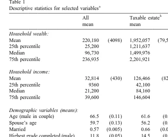
Table 1
Mean 220,180 (4098) 1,952,057 (79,518) 167,734 (1945)
25th percentile 25,200 1,211,637 23,337
Median 96,730 1,499,976 91,000
75th percentile 236,935 2,201,921 217,000
Household income:
Mean 32,814 (430) 126,466 (8201) 29,541 (308)
25th percentile 9360 42,100 9000
Median 21,200 84,160 20,000
75th percentile 39,600 146,604 37,080
Demographic variables(means):
Age (male in couple) 66.5 (0.11) 61.6 (0.48) 66.6 (0.11)
Spouse’s age 59.7 (0.13) 56.2 (0.54) 59.9 (0.13)
Married 0.57 (0.005) 0.66 (0.025) 0.56 (0.005)
Highest grade completed (male) 11.8 (0.05) 14.5 (0.13) 11.7 (0.05)
Nonwhite 0.15 (0.003) 0.04 (0.011) 0.16 (0.003)
Number of children 3.18 (0.017) 2.93 (0.086) 3.19 (0.018) Number of grandchildren 4.86 (0.048) 2.80 (0.183) 4.93 (0.049) Average age of children 37.8 (0.11) 32.1 (0.46) 38.0 (0.11)
c
Average income of children 36,921 (194) 40,329 (1044) 36,798 (197)
d
Number of observations 11,702 360 11,345
a
(Standard errors in parentheses).
b
Assets greater than $600,000 if single, 1.2 million if married.
c
Calculated for non-coresident children only.
d
The number of observations differ for some variables due to missing values.
(including housing wealth) for the entire sample is $220,180. Because wealth is a critical component in the analysis, I also report the 25th, 50th, and 75th percentile points. As is well known from other studies, wealth holdings of the population are highly skewed. Median household wealth is $96,730, less than half of mean wealth. Among the most wealthy households mean wealth is $1,952,057 and the median value is $1,499,976. Similar patterns exist for income.
The number of potential recipients is likely to be an important factor in explaining transfer behavior. The mean number of children for these respondents is 3.2 but is lower for the wealthy than the less wealthy. The wealthy also have fewer grandchildren than do the less wealthy, in part because of the difference in the average age of children. Consistent with the age difference of respondents, children of wealthier parents are 6 years younger on average than children of the less wealthy and are therefore less likely to have completed their childbearing. Despite the age difference, children in the wealthy group have higher incomes.
13
Mean family income for the non-coresident children of wealthy parents is
14
$40,329 compared to $36,798 for the less wealthy.
4. Do taxes affect giving by the wealthy?
In this section I ask how transfer patterns differ between those with bequeath-able wealth above and below the taxbequeath-able levels. If wealthy parents are seeking to avoid estate taxes one would expect to see an increase in both the probability and amount of transfers as wealth increases above $600,000 for a single individual or $1.2 million for a married couple. One would also expect that transfers made by those with taxable levels of bequeathable wealth would be more likely to be made in multiples of $10,000 as permitted by the tax-free limits on gifts, rather than in amounts corresponding to the specific needs of children. In this section I first describe the patterns of transfer behavior evident in the data and then estimate the effect of taxable wealth on transfers in a multivariate context. This latter framework allows me to control for confounding factors such as parental income and the financial status of children.
4.1. Transfer probabilities
In Table 2 I report probabilities of leaving a bequest and of making inter vivos
13
The HRS does not obtain an income measure for coresident children. In AHEAD, respondents are asked to report earnings for coresident children rather than the family income variable obtained for non-coresident children. In my regression analyses I use a dummy variable to indicate the presence of a coresident child and calculate mean income over only non-coresident children.
14
Table 2
Transfer probabilities and amounts
a
All Taxable estate Non-taxable Mean Std Err Mean Std Err Mean Std Err Bequests(AHEAD respondents only)
Have a legal will (0 / 1) 0.69 0.007 0.96 0.022 0.68 0.007 Probability leave a bequest (0–1) 0.53 0.006 0.89 0.026 0.52 0.006
b
Conditional probability bequest . $10,000 0.75 0.006 0.97 0.011 0.74 0.006
c
Conditional probability bequest.$100,000 0.43 0.008 0.91 0.023 0.41 0.009 Inter vivos transfers(HRS and AHEAD)
Proportion making a transfer 0.31 0.004 0.59 0.026 0.30 0.004 Total given (over positive amounts) $5588 244 $14,828 2735 $4944 179 Total amount is divisible by $10,000 (0 / 1) 0.07 0.004 0.20 0.022 0.06 0.004 Equal transfers to all children 0.11 0.006 0.20 0.031 0.11 0.006 Coefficient of variation for transfers3100 138.4 1.36 109.7 6.18 140.3 1.39
a
Assets greater than $600,000 if single, 1.2 million if married.
b
Conditional on the probability a bequest being greater than zero, unconditional probabilities are 0.54, 0.94, and 0.53.
c
Conditional on the probability of leaving a bequest .$10,000 greater than 0.30, unconditional probabilities are 0.26, 0.88, 0.24.
transfers for the entire sample and separately by wealth category. Respondents in the AHEAD survey were asked to report whether they had a will and the
15
probability of leaving certain amounts. Information on intended bequests was not
obtained in the HRS.
Sixty-nine percent of the sample has a legal will, but there is a substantial difference across wealth groups: 96% of the wealthiest segment of the population had a will compared to 68% of the less wealthy.
Respondents were asked also to report the probability of leaving any bequest, the probability of leaving at least $10,000, and the probability of leaving at least $100,000. Answers were given on a 0 to 100 point scale but I have rescaled the figures to lie between 0 and 1. The mean probability of leaving any bequest is 0.53 for the entire sample, and 0.89 among the wealthy. Those who reported a non-zero value for the probability of leaving an inheritance were asked to report the probability of leaving a bequest of $10,000 or more. Virtually all the wealthy expect to bequeath at least this much, with the mean probability being 0.97. Among the less wealthy the conditional probability of bequeathing $10,000 or
15
more is a good deal lower at 0.74. (The two probabilities fall to 0.94 and 0.53 if those who were not asked the question were assigned a probability of zero.) The final question, the probability of leaving $100,000 or more, was asked of those with a reported value of 0.30 or greater for the $10,000 question. Here again the wealthy gave responses near one. The conditional probabilities for the wealthy and less wealthy are 0.91 and 0.41. The unconditional probabilities are 0.88 and 0.24. Given the certainty the wealthy attach to large bequests, it is likely that the eventual inheritances are, at least in part, expected. One would therefore expect a prudent parent to give some consideration to the tax consequences of her giving and to behave so as to reduce the fraction of the estate lost to taxes.
In the lower portion of Table 2 I look for evidence that the wealthy act to reduce estate taxes by making early bequests. The table reports the proportion of families making an inter vivos transfer and the amount transferred. The transfer questions in each survey ask respondents to report transfers of $500 or more made in the past year to any child. While 31% of the families in the sample made transfers of $500 or more to at least one child, this figure jumps to 59% among those with
16
potentially taxable estates. As might be expected, there is also a large difference
in the amount of the transfer by wealth level. The average amount given by those making a transfer is $5,588 for the sample as a whole compared to $14,828 among the wealthy subsample.
Because tax-free giving is restricted to $10,000 per person per year, one might expect those attempting to spend down an estate to be bound by this limit and to make transfers in $10,000 lots. While 20% of the wealthy made transfers that were divisible by $10,000, only 6% of the less wealthy did so.
The final row of Table 2 reports the fraction of families with two or more children in which equal transfers are made to all children. Consistent with the early bequest hypothesis, there is a substantially higher probability of making equal inter vivos
17
transfers for the wealthy group. Just over 20% of those with assets above the
18
taxable limit made equal (non-zero) transfers to all their children in the past year,
16
This figure is higher than that reported in some earlier studies because the sample includes coresident children.
17
These results are not sensitive to requiring exactly equal gifts. When parents differentiate across children the differences are typically large. Among those with potentially taxable estates who made unequal transfers, the mean difference between the highest and the lowest amount is $6739 and the median is $3000. For the less wealthy the mean and median differences are $3107 and $1500. In only 13 families was the difference between children unequal and less than $200.
18
19
compared to 11% of the less wealthy parents. The degree of inequality also
differs across the distribution. Using the coefficient of variation (cv) for transfers to all children within the family as a summary measure, inequality is significantly
20
lower for those with taxable estates than for those with less wealth.
4.2. Multivariate analyses
As shown in Table 1, there are a number of factors that differ significantly by wealth classification. To test the effect of a taxable estate while controlling for these other differences, I turn to multivariate analyses. Table 3 reports the results from regression analyses examining inter vivos giving and intended bequest behavior. The first set of estimates reports the results from a probit model for the probability a transfer is made and the second equation examines the amount of the transfer in a tobit specification. The third and fourth columns report non-linear regression estimates for inheritances, examining the probability of leaving an inheritance, and the probability that the amount bequeathed is greater than $100,000. The sample sizes for this latter pair of regressions differ markedly from those for inter vivos transfers because information on intended bequests is
21
available only for the AHEAD respondents.
One of the important factors that will affect a parent’s decision to spend down her estate is the length of time over which she has to do so. Instead of controlling for the remaining length of life with age, I construct a measure of family life expectancy using 1992 life tables that differ by age, race, and sex (U.S. Department of Health and Human Services, 1996). Each member of a couple may make estate-reducing transfers of up to $10,000 per recipient per year, so it is the combined number of years of life remaining for the couple that is relevant for analyzing transfer behavior. I therefore sum the life expectancies of the two individuals to obtain a measure of the expected number of years the couple has to divest itself of taxable wealth. The mean value of this variable for the entire sample is 29.9. Because the wealthier are younger and more likely to be married, total life expectancy is higher for this group at 37.4 than for the less wealthy, 29.7. This difference underestimates the difference in life expectancy between the two groups since there are known to be significant differences in age-specific mortality
19
For coresident children a sizable portion of their transfer may be in the form of shared food and housing. Thus, parents may be making what they consider to be equal transfers to a coresident and a non-coresident child even if the cash amounts differ. If I exclude coresident children from the calculation, approximately 27% of higher wealth, and 12% of lower wealth families make equal transfers.
20
For the entire sample the correlation between the cv and wealth is 20.11 (not shown) and is significantly different from zero at the 1% level.
21
K
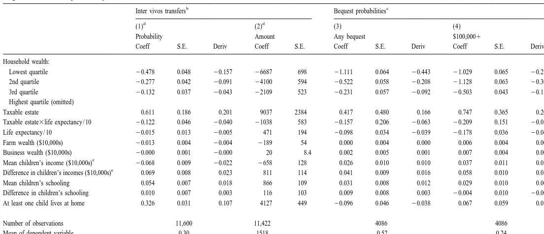
Regressions for the probability and amount of transfer
b c
Inter vivos transfers Bequest probabilities
d d
(1) (2) (3) (4)
Probability Amount Any bequest $100,0001
Coeff S.E. Deriv Coeff S.E. Coeff S.E. Deriv Coeff S.E. Deriv
Household wealth:
Lowest quartile 20.478 0.048 20.157 26687 698 21.111 0.064 20.443 21.029 0.065 20.275 2nd quartile 20.277 0.042 20.091 24100 594 20.522 0.058 20.208 21.128 0.063 20.302 3rd quartile 20.132 0.037 20.043 22109 523 20.231 0.057 20.092 20.503 0.043 20.134 Highest quartile (omitted)
Taxable estate 0.611 0.186 0.201 9037 2384 0.417 0.480 0.166 0.747 0.365 0.200 Taxable estate3life expectancy / 10 20.122 0.046 20.040 21038 583 20.157 0.206 20.063 20.209 0.151 20.056 Life expectancy / 10 20.015 0.013 20.005 471 194 20.098 0.034 20.039 20.178 0.036 20.048 Farm wealth ($10,000s) 20.013 0.004 20.004 2189 54 0.000 0.004 0.000 0.006 0.004 0.001 Business wealth ($10,000s) 20.000 0.001 20.000 20 8.4 0.002 0.005 0.001 0.007 0.004 0.002
e
Mean children’s income ($10,000s) 20.068 0.009 20.022 2658 128 0.026 0.010 0.010 0.037 0.011 0.010 e
Difference in children’s incomes ($10,000s) 0.069 0.008 0.023 811 114 0.041 0.009 0.016 0.058 0.010 0.015 Mean children’s schooling 0.054 0.007 0.018 866 109 0.031 0.008 0.012 0.029 0.010 0.008 Difference in children’s schooling 0.010 0.007 0.003 116 103 0.009 0.008 0.003 20.004 0.010 20.001 At least one child lives at home 0.326 0.031 0.107 4127 449 20.096 0.046 20.038 0.067 0.059 0.018
Number of observations 11,600 11,422 4086 4086
Mean of dependent variable 0.30 1518 0.52 0.24
a
Additional parental characteristics included in the regressions but not shown are: marital status, number of children, number of grandchildren, income quartiles, race, schooling, poor health, and mean children’s income missing.
b
Probability estimated with a probit model, amount estimated with a tobit specification.
c
Probabilities in each column reported on a scale of 0–100, scaled to lie in the range 0–1. Equations estimated using a normal transformation and non-linear least squares. Estimated for AHEAD families only.
d
The number of observations differs from Eq. (1) to Eq. (2) because of missing values on the amount of the transfer.
e
rates by socioeconomic status (Kitagawa and Hauser, 1973; Caldwell and
22
Diamond, 1979; Rosen and Taubman, 1979). Income and wealth are entered into
the regressions in quartiles to allow for non-linear effects and to reduce the influence of outliers. The results are similar for other specifications (see footnote 23). The remainder of the variables in the regressions are readily interpretable.
The effects of the children’s characteristics in these equations are similar to those reported elsewhere (McGarry, 2000). I therefore focus my discussion on the unique aspect of this study, that of the effect of taxable wealth on behavior. As shown in Eq. (1) in Table 3, parental wealth is positively related to the probability of a transfer; moving from the midpoint of the first quartile to the midpoint of the second quartile corresponds to a change of $48,365 in wealth, and an increase of 7 percentage points in the probability of a transfer; a change of 0.14 percentage points per thousand dollars.
The effects of variables indicating a potentially taxable estate are consistent with tax avoidance behavior. In addition to the direct effect of wealth, there is a sharp increase in the probability of a transfer when moving to the portion of the distribution with potentially taxable estates. The direct effect of a taxable estate is an increase of 20 percentage points in the probability. This effect decreases with
the expected length of life (taxable estate 3 life expectancy) as one would expect
if transfers were used to spend down an estate and avoid taxes. Including this interaction term, the net effect of a taxable estate, evaluated at the mean life
23
expectancy (37.4) is 5 percentage points. Note that for the non-wealthy life
24
expectancy has no effect on inter vivos giving.
Various components of wealth may have differential effects on transfer behavior. In particular, wealth in the form of business or farm equity is likely to be less liquid than financial assets and therefore more difficult to transfer. Further-more, these forms of wealth are subject to different treatment with respect to estate
25
taxation than are other assets. In the equation for the probability of a transfer,
22
Poterba (1997) draws attention to the importance of the choice of life table when estimating the eventual estate. When a life table more appropriate for high wealth individuals is used he estimates expected estate taxes that are approximately 30% lower than those calculated with a population life table.
23
The results presented here are similar to those obtained with alternative specifications of wealth, including piecewise linear splines for wealth (and income) and fourth degree polynomials. For example, with the spline specification the direct effect of a taxable estate on the probability of a transfer is an increase 18 percentage points. Each additional year of life expectancy decreases this derivative by 0.0048. I present the quartile estimates here rather than the splines because the estimated effects and combinations are more easily read from the table.
24
As an informal test of whether the data exhibit a true ‘‘break’’ in transfer behavior at the $600,000 limit, I conducted a specification search by varying the amount of wealth used to define the indicator variable. I tested $100,000 intervals between $400,000 and $1 million (or twice that for married couples) and compared the value of the log likelihood for each estimated equation. By this measure the best fit was at $500,000, but the improvement was small relative to the value at $600,000.
25
business wealth does not have a differential effect, but wealth tied up in a farm is less likely to generate transfers than wealth held in other forms. For someone in the highest wealth quartile, an additional $100,000 in farm wealth reduces the probability of a transfer by 4 percentage points.
Income effects (not shown) demonstrate the same monotonic trend as does wealth. To gain further insight into whether the strong relationship between transfers and a taxable estate is simply a non-linear wealth effect, I also experimented with including a dummy variable equal to one if the respondent was in the top 3% of the income distribution, paralleling the dummy variable indicating high wealth. Contrary to the effect of extremely high wealth, the effect of the high income dummy variable was not significantly different from zero.
In addition to tax-driven transfers, parents may also make inter vivos transfers to differentiate across children or to alleviate liquidity constraints on the part of the child. Consistent with the liquidity constraint motivation, the mean income of
26
children has a negative and significant impact on transfers. To capture
differ-ences in income across children to which parents might wish to respond, I include the difference between the incomes of the highest and lowest income child. The probability of a transfer increases with this difference.
The results for the total amount of transfers made (Eq. (2)) are similar to those for the probability of a transfer. The amount of the transfer increases monotonical-ly with both wealth and income. There is also a large and significant effect of having a potentially taxable estate. Those with taxable wealth holdings transfer $9037 more than those with slightly fewer assets. Again the effect is mitigated by length of life. Evaluated at mean life expectancy of wealthy families the additional amount transferred by the wealthiest segment of the population is $5156.
Mean income of the children significantly reduces the amount of the transfer. A $10,000 increase in mean income reduces the amount by $658. A greater difference between the incomes of the highest income and lowest income children is associated with significantly larger transfers.
The third and fourth equations of Table 3 examine bequest behavior. The left hand side variables are responses to questions that asked the respondent to report the probability with which she expects to leave an inheritance and the probability
27
of leaving an estate of $100,000 or more (scaled to lie between 0 and 1). Because the dependent variable is constrained to lie between zero and one, I use a normal
transformation so that Prob(bequest)5F(X9b)1u, and estimate the model using
26
I remind the reader that the children’s income measures are calculated over non-coresident children only. A dummy variable indicating the presence of a coresident child is included and is correlated with a significantly greater probability of a transfer. The results are similar if coresident children are omitted from the analysis.
27
non-linear least squares. Contrary to the results for inter vivos transfers, in neither equation is there a significant effect of having a taxable estate on the probability, nor does the interaction with expected length of life have significant explanatory power. Furthermore, when evaluated at mean life expectancy, the net effects are
negative and close to zero, 20.06 for the probability of a bequest and 20.009 for
the probability of leaving $100,000 or more.
The sharp increase in the probability of transfers and in the amount transferred as one crosses the tax threshold and the lack of an effect on bequest behavior is consistent with the hypothesis that the differing behavior for the wealthy is due to tax laws, and not simply a wealth effect.
5. Taxes and identical transfers
The evidence in the above section suggests that the transfer behavior of the wealthiest segment of the population is altered by the potential tax cost of leaving a very large estate. In this section I examine the degree to which parents take advantage of the opportunity to spend down assets, and consider the trade-off between tax obligations and the psychic cost of making unequal transfers.
5.1. The potential to dissave
Consistent with results reported elsewhere (Poterba, 1998), few in the sample appear to be taking full advantage of the potential to spend down their estates. Even among the wealthiest the vast majority of parents make transfers of less than
g to each child (where g is the maximum tax-free amount permitted to the child1 1
with the smallest family size). There is, however, a significant fraction transferring exactly $10,000 to each child. Among the wealthy, close to 8% of those making transfers made transfers equal to this amount. In contrast only 3% of wealthy
families made transfers of g to each child. Perhaps surprisingly there are almost1
no families (0.9%) in which total transfers exactly equaled the maximum possible tax-free amount, although a substantial fraction appear to have sufficiently high levels of wealth that their estates are likely to incur taxes eventually. Although it is often advantageous to make taxable inter vivos gifts (amounts above $10,000 per person) (Poterba, 1998) only 4% of the wealthy sample made transfers above what
28
appears to be the tax free maximum.
28
5.2. Probability of equal transfers
The frequency of equal transfers among the high wealth group (Table 2), and the rarity with which parents transfer the maximum permitted by law, suggest that they may be more interested in maintaining equal division of their assets than in minimizing the tax owed on the estate. However, it may also be the case that the parents believe they have sufficient time over which to dispose of assets and need not take full advantage of permitted tax-free giving. In this case, among those with potentially taxable estates it would be the very wealthiest who would be most likely to find it necessary to maximize transfers even if it meant differentiating among children. Similarly, holding wealth constant, one might expect those with few years of life remaining, or in poor health to be more likely to make unequal transfers.
Looking first at differences by wealth, I find little evidence that parents with the very highest levels of wealth are less likely to make equal transfers. Fig. 1 plots the probability of equal transfers by wealth category. Equal giving peaks in the range $700,000–$900,000 and then falls by a small (and insignificant) amount
29
before increasing again.
To control for other factors that may be correlated with wealth and with the
Fig. 1. Percent equal transfers by wealth.
29
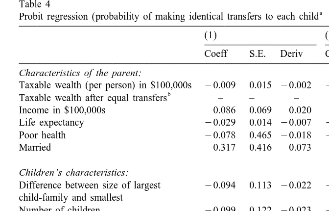
propensity to make equal transfers, I estimate a probit model for the probability of equal treatment, and include wealth, life expectancy, and an indicator of poor health, as explanatory variables. In addition, I include in the regression a measure of income; higher income signals that parents need to draw less on savings to finance their own consumption and must therefore give away more, all else held constant. I also include the number of children because those with more children can divest themselves of more assets in any given year without resorting to unequal gifts, and the difference in family size between the child with the largest and the child with the smallest family. This latter variable captures the potential importance of different transfers; if there is only a small difference in family size there may be little to be saved in taxes by treating children unequally. In addition to tax-motivated transfers, parents whose children have very different income levels may wish to respond to these differences with different levels of transfers. I therefore include measures of the mean income of children and the difference between the income of the highest and lowest income child in the family.
The model is estimated over those families with taxable estates, who have more than one child, and who made at least one transfer in the past year. Those making no transfers are not counted as treating children equally. With these restrictions my
30
sample size falls to 167. Because of the small sample size I interpret the results
31
with caution, and note that many of the coefficients are estimated imprecisely. The results of the analysis are presented in Table 4. Here the measure of wealth is the amount which must be disposed of by each parent if taxes are to be avoided. That is, the wealth variable is the value of assets above the tax-free limit ($600,000 or $1.2 million), divided by two for a married couple. The estimates show little difference in the behavior of the very wealthiest. A $100,000 increase in wealth decreases the probability of equal giving by 0.2 percentage points and
32
the effect is not significantly different from zero.
Contrary to what one would expect, income has a positive effect on the probability of equal transfers, although the estimated effect is small and not statistically significant. The number of years of expected life remaining has significant explanatory power but it too operates in the opposite direction to that predicted by a tax avoidance strategy. Additional years of life imply less urgency in spending down and ought therefore to be associated with a higher probability of equal treatment. Here, however, the effect is negative. Even differences across
30
If I exclude coresident children, the sample size fall to 127 but the results are qualitatively unchanged.
31
Similar estimates of the probability of equal transfers for the entire population are reported in McGarry (2000). For the less wealthy, differences in the amount of inter vivos transfers to children will be driven by differences in the well-being of children. Thus, in contrast to the results presented here, in regressions including the less wealthy, differences in the incomes of children have strong effects on the probability of equal giving.
32
Table 4
a
Probit regression (probability of making identical transfers to each child
(1) (2)
Coeff S.E. Deriv Coeff S.E. Deriv Characteristics of the parent:
Taxable wealth (per person) in $100,000s 20.009 0.015 20.002 20.012 0.016 20.003
b
Taxable wealth after equal transfers – – – 0.359 0.334 0.081 Income in $100,000s 0.086 0.069 0.020 0.077 0.070 0.018 Life expectancy 20.029 0.014 20.007 20.028 0.014 20.006
Poor health 20.078 0.465 20.018 20.109 0.468 20.025
Married 0.317 0.416 0.073 0.273 0.423 0.062
Children’s characteristics:
Difference between size of largest 20.094 0.113 20.022 20.112 0.115 20.025 child-family and smallest
Number of children 20.099 0.122 20.023 20.053 0.128 20.012
c
Mean children’s income ($10,000s) 0.118 0.083 0.027 0.127 0.084 0.029
c
Difference in children’s incomes ($10,000) 20.092 0.073 20.021 20.104 0.075 20.023 At least one child lives at home 20.579 0.302 20.134 20.651 0.313 20.147
Number of observations 167
Mean of the dependent variable 0.22
a
Sample is families with two or more children, who made at least one transfer. Regression also includes a dummy variable for mean children’s income missing and a constant term.
b
Variable equal one if the parent(s) will have wealth.600,000 per person after transfers of g to all1
children.
c
Calculated over non-coresident children.
children in their potential to receive tax-free gifts (( gn2g ) / 10,000) does not1
significantly affect equal giving, although the direction of the effect is as expected. It may be that the effect of wealth occurs at only very high levels. To test for this non-linearity, I re-estimated the equation for the probability of equal transfers including a dummy variable indicating whether the parent could spend down sufficiently by treating children equally (i.e., an indicator of whether wealth is greater than $600,0001( g13n3e)). The results are reported in the second set of
estimates in Table 4. The high wealth indicator is not significantly different from zero and operates in the direction opposite of that predicted.
The lack of a significant relationship between the wealth of parents and equal transfers, and the counterintuitive effects of income and life expectancy, suggest that while parents may be willing to make inter vivos transfers to spend down an estate, they do not do so to the extent that it means treating children unequally.
5.3. Potential tax savings
forecast the wealth trajectories of the respondents in my sample, I cannot address
33
this issue fully. I can, however, calculate the potential to reduce taxes.
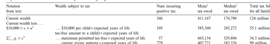
Table 5 reports the imputed tax liability for the respondents in my sample. The table shows the number of families incurring a positive tax bill, and the mean and
34
median amounts paid under various assumptions about inter vivos giving. In the
first row I assume that no gifts are made and calculate the tax bill for current wealth holdings. In this case the 346 families with taxable wealth will owe $124
35
million. The mean amount owed by a family is $411,167 and the median is
$174,780. The second row assumes that parents give each of their children $10,000 per year for every remaining expected year of life ($20,000 per year for a couple as long as both spouses are alive and $10,000 per year after the death of one spouse). The total owed in estate taxes falls by more than half to $55.1 million to be shared by 105 families. Thus even with this simplest method of estate planning the tax burden can be reduced substantially. In the third row, if parents acted solely to avoid estate taxes and transferred the maximum amount permitted to each child in each year, only 57 families would be expected to owe a tax and their total tax bill would be cut to $34.3 million.
How close does the transfer behavior of parents come to these various schemes? In the last row of the Table 1 assume that parents repeat their current transfer patterns for the remaining years of their lives. Under this assumption, 279 families will be left with taxable wealth and a total tax bill of $99 million. Comparing the two bottom rows, parents are foregoing a large tax savings by making fewer transfers than are permitted. By simply maximizing spend-down parents could reduce the aggregate tax bill by 65%.
These numbers undoubtedly overstate the tax burden. Parents will consume much of their wealth themselves during their retirement years, and will likely make charitable gifts that reduce their taxable wealth both while they are alive, and through their bequests. To take a specific example, suppose a 70 year old male with $1.5 million deccumulates his wealth at a rate of 3% per year (including any
36
inter vivos transfers). After 12 years (his approximate life expectancy) he will
33
See Poterba (1997) for a similar exercise that provides population totals. His study using the SCF reaches similar conclusions; wealthy parents fail to take full advantage of the potential to spend down their estates.
34
I use the estate tax schedules from Internal Revenue Service (1997a) and do not make any allowances of deductions such as charitable giving. I assume that couples divide the tax burden across their individual estates so as to minimize taxes owed.
35
As shown in Table 1, there are 360 families with potentially taxable estates. Fourteen of these are missing from this table either because they have missing information on the number of children, marital status of any of their children, or number of offspring of any child.
36
McGarry
/
Journal
of
Public
Economics
79
(2001
)
179
–
204
201
Table 5
Imputed tax bills under alternative assumptions about giving
a a
Notation Wealth subject to tax Num incurring Mean Median Total tax bill
from text positive tax tax owed tax owed for all families
Current wealth 346 411,167 174,780 124 million
Current wealth less . . .
b
$10,0003e3n . . . $10,000 per child3expected years of life 105 585,360 245,272 55.1 million tax-free amount to a child)3expected years of life
n b
oi51gi3e . . . maximum permitted tax-free3expected years of life 57 665,134 329,804 34.3 million . . . current giving patterns3expected years of life 279 407,771 183,326 99 million
a
Mean and median are calculated over positive amounts.
b
have reduced his assets to $1.04 million, and need only to divest himself of an
37
additional $440,000.
6. Conclusion
The decisions surrounding estate planning are complicated. Despite earlier work that questions the existence of a bequest motive Hurd (1989, 1997), as shown here and elsewhere (Kotlikoff and Summers, 1981; Gale and Scholz, 1994), a significant amount of wealth is being transferred to heirs, particularly in wealthy families. Parents obviously care for their children and wish to share with them some of their wealth. However, decisions of how much to transfer, when to make transfers, and how much to give to each child, are complicated. Parents appear to want to treat children equally with respect to bequests, perhaps signaling their equal affection for all children. However, as the standard altruism model predicts, a parent’s resources may be more efficiently allocated by providing greater assistance to less well-off children. The tax code adds a further complication to the dilemma faced by parents. If parents leave ‘‘too much’’ to their children (more than $600,000) the government taxes the excess. Parents can avoid much of the potential tax by making bequest-based transfers before their deaths. In efficiently transferring resources to avoid taxes parents are again faced with a difficult decision. They must decide whether avoiding taxes is sufficiently important that they are willing to compromise on their desire to will (or transfer early) equal amounts to all children.
This paper demonstrates that the elderly do respond to tax incentives and make ‘‘early bequests.’’ However, there is little evidence to suggest that the elderly deviate from their practice of equal treatment of children or act purely to minimize estate taxes. They seldom go beyond gifts of $10,000 per child and do not come close to the maximum possible tax-free giving. The foregone tax savings is substantial. Moving from current patterns of giving to behavior that maximizes tax-free giving reduces the aggregate tax bill by 65% for this sample. If psychic costs are driving equal giving then these costs are high relative to the financial incentives.
Future work ought to provide a model of savings and consumption in order to forecast more accurately eventual estates. By better approximately the remaining wealth when the parent dies we can better assess the extent to which the wealthy elderly are paying ‘‘too much’’ in taxes. It will also be of interest to note the extent
37
to which estate planning and strategic giving become better targeted as the end of life draws near. Finally, as panel data become available, actual bequests will eventually be observed and the amounts of actual inheritances can then be compared with the tax limits and with the individual’s history of inter vivos giving.
Acknowledgements
This paper was prepared for the ISPE Conference on Bequests and Wealth `
Taxation, University of Liege, Belgium, May 1998. I thank Wei-Yin Hu, Michael Hurd, the editor, and two anonymous referees for helpful comments. Financial support from the Brookdale Foundation and from the National Institute on Aging through grant number AG14110-02 is gratefully acknowledged.
References
Altonji, J.G., Hayashi, F., Kotlikoff, L., 1992. The effects of income and wealth on time and money transfers between parents and children. Mimeo, Northwestern University, March.
Altonji, J.G., Hayashi, F., Kotlikoff, L., 1997. Parental altruism and inter vivos transfers: Theory and evidence. Journal of Political Economy 105 (6), 1121–1166.
Barro, R.J., 1974. Are government bonds net wealth. Journal of Political Economy 82 (6), 1095–1117. Becker, G., Tomes, N., 1979. An equilibrium theory of the distribution of income and intergenerational
mobility. Journal of Political Economy 87 (6), s143–s162.
Bernheim, B.D., Shleifer, A., Summers, L.H., 1985. The strategic bequest motive. Journal of Political Economy 93 (6), 1045–1076.
Bernheim, B.D., Severinov, S., 1998. Bequests as signals: An explanation for the equal division puzzle, unigeniture, and Ricardian non-Equivalence. Mimeo, Stanford University.
Caldwell, S., Diamond, T., 1979. Income differentials in mortality – preliminary results based on IRS-SSA linked data. In: Delbone, L., Scheuren, F. (Eds.), Statistical Uses for Administrative Records with Emphasis on Mortality and Disability Research. U. S. Social Security Administration, Washington, DC, pp. 51–59.
Cox, D., 1990. Intergenerational transfers and liquidity constraints. Quarterly Journal of Economics 105 (1), 187–217.
Davies, J., 1981. The relative impact of inheritance and other factors on economic inequality. Quarterly Journal of Economics 97 (3), 471–498.
Dunn, T., Phillips, J., 1997. Do parents divide resources equally among children? Evidence from the AHEAD survey. Aging Studies Program Paper No. 5, Syracuse University.
Gale, W., Scholz, J.K., 1994. Intergenerational transfers and the accumulation of wealth. Journal of Economic Perspectives 8 (4), 145–160.
Hurd, M., 1987. Savings of the elderly and desired bequests. American Economic Review 77 (3), 298–312.
Hurd, M., 1989. Mortality risk and bequests. Econometrica 57 (4), 779–813.
Internal Revenue Service, 1997a. Introduction to Estate and Gift Taxes. Department of the Treasury, publication 950, June.
Internal Revenue Service, 1997b. Statistics of Income Bulletin. Winter 1996–1997.
Kitagawa, E., Hauser, P., 1973. Differential Mortality in the United States: A Study in Socioeconomic Epidemiology. Harvard University Press, Cambridge, MA.
Kotlikoff, L.J., Summers, L., 1981. The role of intergenerational transfers in aggregate capital accumulation. Journal of Political Economy 89 (4), 706–731.
`
Laferrere, A., Arrondel, L., 1998. Bequest motives and estate taxation in France. In: ISPE Conference `
on Bequests and Wealth Taxation, University of Liege, Belgium.
Masson, A., Pestieau, P., 1997. Bequest motives and models of inheritance: A survey of the literature. In: Erreygers, G., Vandevelde, T. (Eds.), Is Inheritance Legitimate? Ethical and Economic Aspects of Wealth Transfers. Springer-Verlag, Berlin.
McGarry, K., 2000. Inter vivos transfers and intended bequests. Journal of Public Economics 77, 321–351.
McGarry, K., Schoeni, R.F., 1995. Transfer behavior in the health and retirement study. Journal of Human Resources 30, s184–s226.
McGarry, K., Schoeni, R.F., 1997. Transfer behavior within the family: Results from the Asset and Health Dynamics Survey. Journals of Gerontology 52 (B), 82–92.
Menchik, P.L., 1988. Unequal estate division: Is it altruism, reverse bequests, or simply noise. In: Kessler, D., Masson, A. (Eds.), Modelling the Accumulation and Distribution of Wealth. Oxford University Press, New York, pp. 105–116.
Poterba, J., 1997. The estate tax and after-tax investment returns. NBER working paper no. 6337. Poterba, J., 1998. Estate and gift taxes and incentives for inter vivos giving in the United States. NBER
working paper no. 6842.
Rosen, S., Taubman, P., 1979. Changes in the impact of education and income on mortality in the US. In: Delbone, L., Scheuren, F. (Eds.), Statistical Uses for Administrative Records with Emphasis on Mortality and Disability Research. US Social Security Administration, Washington, DC, pp. 61–66. US Department of Health and Human Services, 1996. Vital Statistics of the United States, 1992. Vol. II,
Mortality. Hyattsville, MD.