More Flexible Radial Layout
Ulrik Brandes
1Christian Pich
21Department of Computer & Information Science, University of Konstanz
2Chair of Systems Design, ETH Z¨urich
Abstract
We describe an algorithm for radial layout of undirected graphs, in which nodes are constrained to concentric circles centered at the origin. Such constraints are typical, e.g., in the layout of social networks, when structural centrality is mapped to geometric centrality or when the pri-mary intention of the layout is the display of the vicinity of a distinguished node. Our approach is based on an extension of stress minimization with a weighting scheme that gradually imposes radial constraints on the inter-mediate layout during the majorization process, and thus is an attempt to preserve as much information about the graph structure as possible.
Submitted:
December 2009
Reviewed:
August 2010
Revised:
August 2010
Accepted:
November 2010
Final:
November 2010
Published:
February 2011
Article type:
Regular paper
Communicated by:
D. Eppstein and E. R. Gansner
E-mail addresses:[email protected](Ulrik Brandes)[email protected]
1
Introduction
In radial graph layout the nodes are constrained to lie on a set of concentric circles; for some or all nodes in the graph a radius is given, which typically encodes non-structural information, or the results of a preceding analysis. His-torical examples of such drawings date back to the 1940s [23], and the special case in which all nodes are required to lie on the same circle is a often referred to as circular layout.
We are interested in designing a method to determine layouts that meet the following two, possibly contradicting, criteria:
• Representation of distances: The Euclidean distance between two nodes in the drawing should correspond to their graph-theoretical distance.
• Radial constraints: Nodes are associated with the radius of a circle cen-tered at the origin, and are constrained to be placed on the circumference of this circle.
While the first criterion is a general readability objective in undirected graph layout, the constraints in the second criterion are specific to the application at hand.
An example is the exploration of hierarchies with discrete (nominal-scale) layers [8]; in [25] large such hierarchies are laid out radially as a tree, followed by an incremental force-based placement. This approach was later modified for dynamic real-time exploration of a filesharing network in [26], where users interactively select a node to be moved into the center, triggering an update of the immediate surrounding of that node. A different approach is to adapt the Sugiyama framework, originally designed for layout in parallel layers, to radial layers [1].
In the case of fixed radii defined to represent some continuous (interval-scale) node valuation, unary constraints are imposed on the drawing. This scenarion is introduced in [5] to map any (structural) centrality index to visual centrality. Layouts are determined from a combination of simulated annealing, which is very flexible and allows for penalty costs, e.g., for edge crossings, and force-directed placement. Because of its high computational cost, this method does not scale even to moderately sized graphs, though. For applications in social network analysis, it was therefore replaced by a combinatorial approach based on circular layout [2].
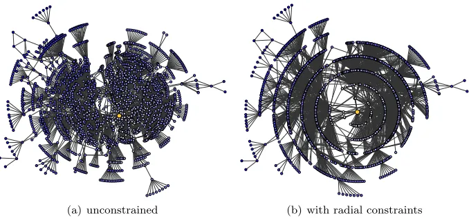
(a) unconstrained (b) with radial constraints
Figure 1: A social network (courtesy of Carola Lipp; 2075 nodes, 4769 edges), consisting of two known clusters. The darkness of nodes is proportional to their distances from the distinguished focal node, which also defines the radii used in the constrained layout. Note that distances are represented more clearly, while the two clusters are apparent, still.
All these approaches modify the targetdistances themselves in one form or another, while the approach presented here is based on engineering theweights
used in the stress minimization model. The weights are coefficients of error terms involved in the quality criteria to be minimized. If chosen carefully, these weights can be used to influence the configuration resulting from optimizing the modified stress function; see Fig. 1 for an example. We are not aware of previous work in graph drawing which systematically adjusts weights to adapt an objective function to meet layout criteria.
2
Preliminaries
LetG= (V, E) be a simple undirected graph, i.e.,E⊆ V2
. We will denote the cardinalities of the node and edge sets by n=|V| and m=|E|, respectively; it is sometimes convenient to index nodes by numbers,V ={v1, . . . , vn}. The
graph-theoretical distance between two nodesu, v is the number of edges on a shortest path betweenuandvand is denoteddu,v or, when there is no danger
of confusion, duv. The matrix D = (duv)uv ∈ Rn×n contains the distances
between every two nodes in G; the diameter of G is the maximum distance between any two nodes inG, diam(G) = maxu,v∈V duv. All graphs are assumed
to be connected; otherwise, connected components are considered individually. Two-dimensional node positions are denoted by p(v) = (xv, yv). The
Eu-clidean distance between two nodes in a layoutpis defined askp(u)−p(v)k= (xu−xv)2+ (yu−yv)2
1/2
3
Stress, Weights, and Constraints
3.1
Stress
The foundation of our method is multidimensional scaling (MDS) [3, 9]. Orig-inating in psychometrics and the social sciences, MDS has been established and widely used for graph drawing since its popularization by Kamada and Kawai [19]. While there is a wide range of variants and extensions, we here concentrate on thestress minimization approach [16].
Given a set of target distances among a set ofnobjects, the overall goal is to place these objects in a low-dimensional Euclidean space in such a way that the resulting distances fit the desired ones as well. In the graph drawing literature, the desired distances are usually graph-theoretical (shortest-path) distancesduv,
and the goal is to find two-dimensional positionsp(v) for all nodesv∈V with
kp(u)−p(v)k ≈duv
attained as closely as possible for all pairs u, v. When the configuration is not required to satisfy any further constraints, the objective function, called (weighted)stress, is the sum of squared residuals
σ(p) =X
There is wide consensus that configurations with a small stress value tend to be structurally informative, and aesthetically pleasing. The state-of-the-art approach to finding such layouts is stress majorization [10, 16]; starting from an initial configuration, it generates an improving sequence of layouts. When no coordinates are at hand, the iterative process may be initialized at random, but more favorable and robust strategies are available. The experiments of [7] indicate that approximate classical scaling [6] is the method of choice.
During stress majorization, new positions ˆp(u) = (ˆxu,yˆu) for every node
u∈V can be computed from the current positions using the update rules
ˆ
criterion. The sequence of layouts generated in this way can be shown to have non-increasing stress and to converge towards a local minimum [11].
3.2
Weights for Constraints
In early applications of MDS, each pairu, v of objects was assigned the same unit weight corresponding towuv = 1 in (1). When a target distance is unknown
for some pair, it is simply ignored by using a zero weight for its contribution to the stress.
The standard weighted scheme for graph drawing useswuv =d−2uv. It was
introduced as elastic scaling by McGee [21], and is equal to the one used by Kamada and Kawai [19]. Its superiority is due to an emphasis of small distances over large ones. This is because the fit of local distances is visually important, but also because it means that instead of fitting absolute values by minimizing
absolute residual error terms
(duv− kp(u)−p(v)k)2 ,
the objective is reformulated inrelative error terms
(1− kp(u)−p(v)k/duv)2 .
Summing these over all pairs gives
X
A reason for the favorable aesthetic properties of low-stress layouts is that no node is preferred over others because minimization of the objective function is an attempt to achieve a balance in the fit of the desired distances. In most scenarios this is appropriate and tends to give the drawing a pleasing appearance.
In some cases, it may be desirable to put more emphasis on some nodes, while other nodes are regarded less important, for instance by centering the view on a node and visualizing this node’s neighborhood more prominently. This can be done by introducing suitable constraints on the configuration. When these constraints can be formulated in terms of target distances, choosing the weights in a suitable way allows to impose them on the resulting layout without changing the layout algorithm.
What follows is a general framework for constrained graph drawing in sce-narios in which constraints can be expressed in terms of target distances. While the range of possible applications is much wider, our contribution will concen-trate on the radial layout scenario. To avoid confusion, objective function (1) will be referred to asdistance stress, denoted byσW(p). The subscript indicates
that the stress defined using weight matrix W = (wuv)uv ∈Rn×n. This stress
model is extended by a second set of weightsZ= (zuv)uvused for theconstraint stress defined by
σZ(p) = X
u,v
Its minimization is an attempt to fit the same distances and hence aims at representing the same information, but highlights different aspects.
3.3
Interpolated Weights
A straightforward approach to satisfy constraints associated with an additional weight matrixZ is to minimize (4) directly, say, after minimization of distance stress σW. This tends, however, to result in trivial solutions. Consider for
instance radial constraints forcing each nodev ∈V to be at distance rv from
the center. Clearly, we may end up in a layout withxv =rv, yv = 0 from any
initial configuration.
Instead, distance and constraint stress should be reduced simultaneously. An effective approach is to combine them into a joint majorization process, operat-ing on a linear combination of the stress measuresσW(p) and σZ(p) changing
gradually in favor of the constraints.
Initially, nodes are allowed to move freely without considering constraints at all, by minimizing justσW(p). Then, constraints are granted more and more
control over the layout by dynamically changing coefficients in this combination, shifting the bias from one criterion to the other [4]. The relative influence of distance and radial components is determined by the coefficients in the linear combination
σ(1−t)·W+t·Z = (1−t)·σW(p) +t·σZ(p). (5)
This is easily incorporated into the stress majorization process by changing update rules (2) and (3) to
ˆ
In the majorization process, radial constraints are enforced neither directly nor immediately, so that the main visual features of the initial configuration can be preserved. The bias is shifted from the distance component towards the radial component by gradually increasingtfrom 0 to 1. When the number of iteration stepsk is fixed, linear interpolation yields values t = 0,k1,2k, . . . ,k−1k ,1. Oth-erwise, the iterative process may simply be repeated with a sequence of values fork converging to 1 from below until the layout is sufficiently stable. Using either variant, in each step, a slightly different objective function is sought to be minimized, and the current iterate preconditions the next step, thus smoothing the sequence of iterates.
In this terminology, an unconstrained MDS problem can be thought of as a special case of a weakly constrained problem, in which the deviation penalty is zero. In our case, arriving att= 1 in (5) turns the weakly constrained problem into a strongly constrained one, provided that the set of constraints can be satisfied, i.e., a solution with zero constraint stress exists. In all other cases, it should be noted that, even though the distance component vanishes when t→1, minimizingσ(1−t)·W+t·Z(p) isnot the same as minimizingσZ(p) because
of the running preconditioning described above.
4
Radial Layout
To illustrate the utilization of radial constraints for interest-based graph layout, we discuss three different scenarios in this section.
4.1
Focusing on a Node
In aneighborhood diagram, the focus is put on a node by distorting its surround-ings. Here we constrain all others to be located at a Euclidean distances from the distinguished node that corresponds to their graph-theoretical distances from it, i.e., the distance-k neighborhood is mapped to thekcircle centered on that node (which can be regarded as the geometrick-neighborhood).
To implement this design, the constraint weight matrix takes those pairs of nodes into account that the focal node, say vi, is involved in, with all other
weights reduced to zero. Matrices D and W are defined as above, and the constraint weight matrixZ = (zuv)uv has non-zero entries only in thei-th row
and column
These are derived from the distances to the focal node, so that interpolating from W toZgradually increases the focal node’s relative impact on the configuration. For dynamic visualization scenarios, an inherently smooth transition be-tween layouts with different foci can be obtained by simply using the interme-diate layouts given by the steps in the majorization process. In the transition from one focus to the other, it is advantageous not to interpolate directly be-tween the two corresponding constraint weight matrices, but to take a detour via the original weight matrix having entriesd−2
uv, so as to re-introduce all the
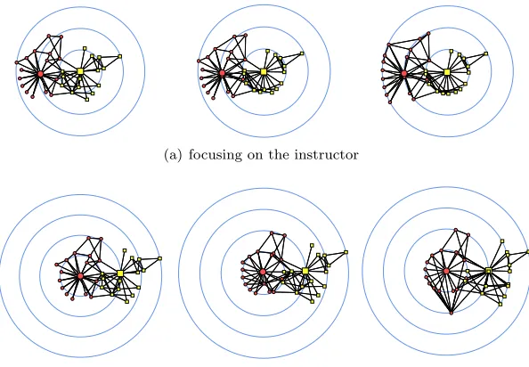
As an example, we consider a famous social network studied by Zachary and, subsequently, many others [27]. It describes friendship relations among 34 members in the karate club of a U.S. university in the 1970s. Over the course of a two-year study, the network breaks apart into two clubs because of disagreements between the administrator and the instructor, with the latter leaving the club and taking about half of the members with him. Following [22], this data set has been used frequently as a benchmark for the performance of various clustering approaches.
(a) focusing on the instructor
(b) focusing on the administrator
Figure 2: Radial layouts of Zachary’s karate club network (n= 34, m= 77), by weight interpolation, fort∈ {0,0.9,1}. Members leaving with the instructor are shown as yellow squares, members staying with the administrator as red circles.
Fig. 2 shows how the same initial layout, which is computed by minimizing stress without constraints, is gradually modified into radial layouts, one focusing on the instructor and the other on the administrator.
The insight gained from Fig 2 is two-fold. Technically, it is visible that large parts of the overall shape of the layout are preserved well during the gradual relative increase of constraint stress. Substantively, we can see immediately that the decision to leave the club is in one-to-one correspondence with the presence in the neighborhood of the instructor or administrator. The only exceptions are the two members in each group that have direct ties with both of them. The two rightmost drawings clearly tell the whole story and also show that practically
4.2
Centrality Drawings
A special property of the constraints in the previous section is that their target distances correspond directly to a column in distance matrixD. In centrality drawings, the requirement is that radii are given as part of the input, and therefore in general do not correspond to the distance from an existing focal node. It is, however, easy to augment the distance matrix accordingly.
Assume that nodes are numbered v1, . . . , vn and that the radii are given
as additional input in a vector r = [r1, . . . , rn]T ∈ Rn, with ri ≥ 0 for all
i= 1, . . . , n. Since radial constraints can be specified in terms of distances from the origin, we express then as
kp(vi)k=ri .
This way the origin can be incorporated as a dummy nodevn+1 with artificial target distancesdvi,vn+1=dvn+1,vi =ri, and the stress majorization procedure
is applied to a layout problem ofn+ 1 objects. Such a dummy is used, e.g., in [4] to enforce a circular configuration by using the same radius for all objects. Distance and weight matrices are set up for (5) as
D =
Algorithm 1:Layout with general radial constraints
Input: connected undirected graphG= (V, E),
radiirv ∈R>0 for allv∈V, number of iterationsk∈N
Output: coordinatesp(v) withkp(v)k=rv for allv∈V
D←matrix of shortest path distancesduv
W ←matrix of inverse squared distancesd−2
uv
to emphasize the structure in different centrality intervals. For instance, the central (peripheral) areas are enlarged by applying a concave (convex) function magnifying regions of smaller (larger) centrality scores.
Examples of centrality drawings for Zachary’s karate club network are shown in Figure 3. The left column is based oncloseness centrality [24]
cv= X1
t∈V
dvt
,
which is simply the inverse average distance from a vertex to all others. The right column contains drawings based onbetweenness centrality [14]
cv= X
s6=v6=t∈V
δ(s, t|v),
where δ(s, t|v) is the dependency of s, t ∈ V on v ∈ V, which is defined as the fraction of shortest (s, t)-paths that contain v as an inner vertex. Not surprisingly, both the instructor and the administrator are central according to any measures. It is interesting to note, however, that this is due to the fact that they integrate largely separate neighborhoods. The layouts reveal that closeness values have a higher resolution in the center, whereas betweenness has more variance in the periphery. These diagrams should not be seen as part of a serious exploration, though, but as mere illustrations of possible use cases.
closeness centrality betweenness centrality
u
n
if
or
m
em
p
h
as
iz
in
g
ce
n
te
r
em
p
h
as
iz
in
g
p
er
ip
h
er
y
Figure 3: Centrality layouts of the karate club social network, using two com-mon centrality measures to define the radii of nodes. Center and periphery are emphasized using transformed radiiri′ = 1−(1−ri)3 and ri′ =r3i (0≤ri≤1
and 0≤r′
where quantitiesav are defined as
Schematic maps have become an essential guide for travelers in public trans-portation systems. Such maps commonly depict lines, stations, zones, and con-nections to other traffic systems. Since the primary use of such maps is for travel planning, usability and readability are more important criteria than the accurate representation of actual geographic positions. In the graph drawing literature, this drawing style is called metro map layout (see, e.g., [18] for a force-directed approach).
The seminal design is Harry Beck’s map of London Underground, commonly known as the Tube. It has been and still is being reworked and improved, and it has inspired similar maps for systems of public transportation all over the world. While schematic maps are widely perceived as very useful, a potential drawback is that they tend to distort a user’s perception of distance, thus poten-tially compromising decisions made in the travel planning process, e.g., because stations are displayed as more proximate than they actually are.
If the starting and ending stations of a planned journey are known, radial constraints can be used to highlight the time needed for traveling between them by focusing only on the starting station as described above. Alternatively, short-est paths between the two stations can be highlighted by putting the focus on both of them at the same time.
Again,D, W ∈Rn×n are defined as the matrices of shortest-path distances
and their inverse squares, respectively. The constraint weight matrix is set to
Z =
wherevn−1andvnare assumed to be the focal nodes. When interpolating from
the original weight matrix W to the constraint weight matrixZ, distances to (and between) the two focused nodes become increasingly influential.
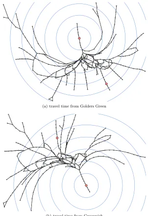
As an example we use a connection graph of the Tube with approximate station locations and travel times.1 Radial layouts are given in Fig. 4, where stations are placed at a distance from the center proportional to their estimated minimum travel times from two sample stations. Since travel times are only approximately related to shortest-path distance, these examples are more closely related to centrality drawings than to neighborhood diagrams.
1Made available by Tom Carden athttp://www.tom-carden.co.uk/p5/tube_map_travel_
Their combination is shown in Fig 5. Even though this map is only an experimental illustration of a scenario with two foci, it does convey a sense of alternate direct routes and detours.
5
Discussion
We argued that radial constraints fit well into the framework of multidimensional scaling by stress majorization with a penalty function.
An obvious advantage is the simplicity of our approach, because radii can be expressed in terms of target distances and thus require only minor modifications of available implementations for stress minimization.
Since the method can be initialized with any layout and constraints are introduced only gradually, we are likely to end up in a feasible solution close to the initial one. While sensitivity to initialization is usually a disadvantage of iterative layout methods, it is very welcome in the present scenario, because it instills hope that some properties of a high-quality unconstrained layout can be preserved in the solution obtained. Together with the greater degree of freedom during most of the process, it is possible that stress majorization with penalty functions is not only simpler, but also more effective than gradient-projection methods [12] which maintain a feasible solution throughout. An in-depth comparison is therefore an important direction for future research.
(a) travel time from Golders Green
(b) travel time from Greenwich
(a) geographically accurate
(b) dual-focus radial layout with circles in 10min intervals
References
[1] C. Bachmaier. A radial adaption of the Sugiyama framework for visual-izing hierarchical information. IEEE Transactions on Visualization and Computer Graphics, 13(3):583–594, 2007.
[2] M. Baur and U. Brandes. Crossing reduction in circular layouts. In J. Hromkoviˇc, M. Nagl, and B. Westfechtel, editors, Proceedings of the 30th International Workshop on Graph-Theoretical Concepts in Computer Science (WG’04), volume 3353 ofSpringer LNCS, pages 332–343, 2004.
[3] I. Borg and P. Groenen. Modern Multidimensional Scaling. Springer, 2005.
[4] I. Borg and J. Lingoes. A model and algorithm for multidimensional scaling with external constraints on the distances. Psychometrika, 45(1):25–38, 1980.
[5] U. Brandes, P. Kenis, and D. Wagner. Communicating centrality in pol-icy network drawings. IEEE Transactions on Visualization and Computer Graphics, 9(2):241–253, 2003.
[6] U. Brandes and C. Pich. Eigensolver methods for progressive multidimen-sional scaling of large data. In M. Kaufmann and D. Wagner, editors, Pro-ceedings of the 14th International Symposium on Graph Drawing (GD’06), volume 4372 of Springer LNCS, pages 42–53, 2007.
[7] U. Brandes and C. Pich. An experimental study on distance-based graph drawing. In Proceedings of the 16th International Symposium on Graph Drawing (GD’08), volume 5417 ofSpringer LNCS, pages 218–229, 2009.
[8] M.-J. Carpano. Automatic display of hierarchized graphs for computer-aided decision analysis. IEEE Transactions on Systems, Man and Cyber-netics, 10(11):705–715, 1980.
[9] T. F. Cox and M. A. A. Cox. Multidimensional Scaling. CRC/Chapman and Hall, 2001.
[10] J. de Leeuw. Applications of convex analysis to multidimensional scaling. In J. R. Barra, F. Brodeau, G. Romier, and B. van Cutsem, editors,Recent De-velopments in Statistics, pages 133–145. Amsterdam: North-Holland, 1977.
[11] J. de Leeuw. Convergence of the majorization method for multidimensional scaling. Journal of Classification, 5(2):163–180, 1988.
[12] T. Dwyer, Y. Koren, and K. Marriott. Constrained graph layout by stress majorization and gradient projection. Discrete Applied Mathematics, 309:1895–1908, 2008.
[14] L. C. Freeman. A set of measures of centrality based on betweenness.
Sociometry, 40:35–41, 1977.
[15] E. R. Gansner and Y. Hu. Efficient node overlap removal using a proximity stress model. InProceedings of the 16th International Symposium in Graph Drawing (GD’08), volume 5417 ofSpringer LNCS, pages 206–217, 2009.
[16] E. R. Gansner, Y. Koren, and S. North. Graph drawing by stress ma-jorization. In Proceedings of the 11th International Symposium in Graph Drawing (GD’03), volume 2912 ofSpringer LNCS, pages 239–250, 2004.
[17] W. J. Heiser and J. Meulman. Constrained multidimensional scaling, in-cluding confirmation. Applied Psychological Measurement, 7(4):381–404, 1983.
[18] S.-H. Hong, D. Merrick, and H. A. D. do Nascimiento. The metro map layout problem. InProceedings of the 2004 Australasian symposium on In-formation Visualisation, ACM International Conference Proceeding Series, pages 91–100, 2004.
[19] T. Kamada and S. Kawai. An algorithm for drawing general undirected graphs. Information Processing Letters, 31:7–15, 1989.
[20] Y. Koren and A. C¸ ivril. The binary stress model for graph drawing. In Pro-ceedings of the 16th International Symposium in Graph Drawing (GD’08), volume 5417 of Springer LNCS, pages 193–205, 2009.
[21] V. E. McGee. The multidimensional scaling of “elastic” distances. The British Journal of Mathematical and Statistical Psychology, 19:181–196, 1966.
[22] M. E. J. Newman and M. Girvan. Finding and evaluating community structure in networks. Physical Review E, 69:026113, 2004.
[23] M. L. Northway. A method for depicting social relationships obtained by sociometric testing. Sociometrics, 3:144–150, 1940.
[24] G. Sabidussi. The centrality index of a graph. Psychometrika, 31:581–603, 1966.
[25] G. J. Wills. NicheWorks – interactive visualization of very large graphs. In Proceedings of the 5th International Symposium in Graph Drawing (GD’97), pages 403–414, 1997.
[26] K.-P. Yee, D. Fisher, R. Dhamija, and M. Hearst. Animated exploration of dynamic graphs with radial layout. InProceedings of the IEEE Symposium on Information Visualization 2001 (InfoVis ’01), pages 43–50, 2001.