Mathematics of the Discrete Fourier Transform
(DFT)
Julius O. Smith III ([email protected])
Center for Computer Research in Music and Acoustics (CCRMA) Department of Music, Stanford University
Stanford, California 94305
Contents
1 Introduction to the DFT 1
1.1 DFT Definition . . . 1
1.2 Mathematics of the DFT . . . 3
1.3 DFT Math Outline . . . 6
2 Complex Numbers 7 2.1 Factoring a Polynomial . . . 7
2.2 The Quadratic Formula . . . 8
2.3 Complex Roots . . . 9
2.4 Fundamental Theorem of Algebra . . . 11
2.5 Complex Basics . . . 11
2.5.1 The Complex Plane . . . 13
2.5.2 More Notation and Terminology . . . 14
2.5.3 Elementary Relationships . . . 15
2.5.4 Euler’s Formula . . . 15
2.5.5 De Moivre’s Theorem . . . 17
2.6 Numerical Tools in Matlab . . . 17
2.7 Numerical Tools in Mathematica . . . 23
3 Proof of Euler’s Identity 27 3.1 Euler’s Theorem . . . 27
3.1.1 Positive Integer Exponents . . . 27
3.1.2 Properties of Exponents . . . 28
3.1.3 The Exponent Zero . . . 28
3.1.4 Negative Exponents . . . 28
3.1.5 Rational Exponents . . . 29
3.1.6 Real Exponents . . . 30
3.1.7 A First Look at Taylor Series . . . 31
3.1.8 Imaginary Exponents . . . 32
Page iv CONTENTS
3.1.9 Derivatives off(x) =ax . . . 32
3.1.10 Back to e . . . 33
3.1.11 Sidebar on Mathematica . . . 34
3.1.12 Back to ejθ . . . 34
3.2 Informal Derivation of Taylor Series . . . 36
3.3 Taylor Series with Remainder . . . 37
3.4 Formal Statement of Taylor’s Theorem . . . 39
3.5 Weierstrass Approximation Theorem . . . 40
3.6 Differentiability of Audio Signals . . . 40
4 Logarithms, Decibels, and Number Systems 41 4.1 Logarithms . . . 41
4.1.1 Changing the Base . . . 43
4.1.2 Logarithms of Negative and Imaginary Numbers . 43 4.2 Decibels . . . 44
4.2.1 Properties of DB Scales . . . 45
4.2.2 Specific DB Scales . . . 46
4.2.3 Dynamic Range . . . 52
4.3 Linear Number Systems for Digital Audio . . . 53
4.3.1 Pulse Code Modulation (PCM) . . . 53
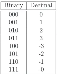
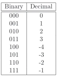
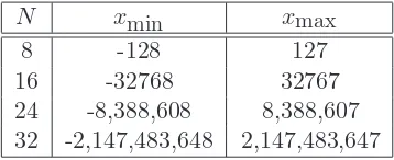
4.3.2 Binary Integer Fixed-Point Numbers . . . 53
4.3.3 Fractional Binary Fixed-Point Numbers . . . 58
4.3.4 How Many Bits are Enough for Digital Audio? . . 58
4.3.5 When Do We Have to Swap Bytes? . . . 59
4.4 Logarithmic Number Systems for Audio . . . 61
4.4.1 Floating-Point Numbers . . . 61
4.4.2 Logarithmic Fixed-Point Numbers . . . 63
4.4.3 Mu-Law Companding . . . 64
4.5 Appendix A: Round-Off Error Variance . . . 65
4.6 Appendix B: Electrical Engineering 101 . . . 66
5 Sinusoids and Exponentials 69 5.1 Sinusoids . . . 69
5.1.1 Example Sinusoids . . . 70
5.1.2 Why Sinusoids are Important . . . 71
5.1.3 In-Phase and Quadrature Sinusoidal Components . 72 5.1.4 Sinusoids at the Same Frequency . . . 73
5.1.5 Constructive and Destructive Interference . . . 74
CONTENTS Page v
5.2.1 Why Exponentials are Important . . . 77
5.2.2 Audio Decay Time (T60) . . . 78
5.3 Complex Sinusoids . . . 78
5.3.1 Circular Motion . . . 79
5.3.2 Projection of Circular Motion . . . 79
5.3.3 Positive and Negative Frequencies . . . 80
5.3.4 The Analytic Signal and Hilbert Transform Filters 81 5.3.5 Generalized Complex Sinusoids . . . 85
5.3.6 Sampled Sinusoids . . . 86
5.3.7 Powers ofz . . . 86
5.3.8 Phasor & Carrier Components of Complex Sinusoids 87 5.3.9 Why Generalized Complex Sinusoids are Important 89 5.3.10 Comparing Analog and Digital Complex Planes . . 91
5.4 Mathematica for Selected Plots . . . 94
5.5 Acknowledgement . . . 95
6 Geometric Signal Theory 97 6.1 The DFT . . . 97
6.2 Signals as Vectors . . . 98
6.3 Vector Addition . . . 99
6.4 Vector Subtraction . . . 100
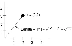
6.5 Signal Metrics . . . 100
6.6 The Inner Product . . . 105
6.6.1 Linearity of the Inner Product . . . 106
6.6.2 Norm Induced by the Inner Product . . . 107
6.6.3 Cauchy-Schwarz Inequality . . . 107
6.6.4 Triangle Inequality . . . 108
6.6.5 Triangle Difference Inequality . . . 109
6.6.6 Vector Cosine . . . 109
6.6.7 Orthogonality . . . 109
6.6.8 The Pythagorean Theorem in N-Space . . . 110
6.6.9 Projection . . . 111
6.7 Signal Reconstruction from Projections . . . 111
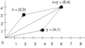
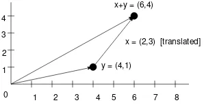
6.7.1 An Example of Changing Coordinates in 2D . . . 113
6.7.2 General Conditions . . . 115
6.7.3 Gram-Schmidt Orthogonalization . . . 119
6.8 Appendix: Matlab Examples . . . 120
Page vi CONTENTS
7 Derivation of the Discrete Fourier Transform (DFT) 127
7.1 The DFT Derived . . . 127
7.1.1 Geometric Series . . . 127
7.1.2 Orthogonality of Sinusoids . . . 128
7.1.3 Orthogonality of the DFT Sinusoids . . . 131
7.1.4 Norm of the DFT Sinusoids . . . 131
7.1.5 An Orthonormal Sinusoidal Set . . . 131
7.1.6 The Discrete Fourier Transform (DFT) . . . 132
7.1.7 Frequencies in the “Cracks” . . . 133
7.1.8 Normalized DFT . . . 136
7.2 The Length 2 DFT . . . 137
7.3 Matrix Formulation of the DFT . . . 138
7.4 Matlab Examples . . . 140
7.4.1 Figure 7.2 . . . 140
7.4.2 Figure 7.3 . . . 141
7.4.3 DFT Matrix in Matlab . . . 142
8 Fourier Theorems for the DFT 145 8.1 The DFT and its Inverse . . . 145
8.1.1 Notation and Terminology . . . 146
8.1.2 Modulo Indexing, Periodic Extension . . . 146
8.2 Signal Operators . . . 148
8.2.1 Flip Operator . . . 148
8.2.2 Shift Operator . . . 148
8.2.3 Convolution . . . 151
8.2.4 Correlation . . . 154
8.2.5 Stretch Operator . . . 155
8.2.6 Zero Padding . . . 155
8.2.7 Repeat Operator . . . 156
8.2.8 Downsampling Operator . . . 158
8.2.9 Alias Operator . . . 160
8.3 Even and Odd Functions . . . 163
8.4 The Fourier Theorems . . . 165
8.4.1 Linearity . . . 165
8.4.2 Conjugation and Reversal . . . 166
8.4.3 Symmetry . . . 167
8.4.4 Shift Theorem . . . 169
8.4.5 Convolution Theorem . . . 171
CONTENTS Page vii
8.4.7 Correlation Theorem . . . 173
8.4.8 Power Theorem . . . 174
8.4.9 Rayleigh Energy Theorem (Parseval’s Theorem) . 174 8.4.10 Stretch Theorem (Repeat Theorem) . . . 175
8.4.11 Downsampling Theorem (Aliasing Theorem) . . . 175
8.4.12 Zero Padding Theorem . . . 177
8.4.13 Bandlimited Interpolation in Time . . . 178
8.5 Conclusions . . . 179
8.6 Acknowledgement . . . 179
8.7 Appendix A: Linear Time-Invariant Filters and Convolution180 8.7.1 LTI Filters and the Convolution Theorem . . . 181
8.8 Appendix B: Statistical Signal Processing . . . 182
8.8.1 Cross-Correlation . . . 182
8.8.2 Applications of Cross-Correlation . . . 183
8.8.3 Autocorrelation . . . 186
8.8.4 Coherence . . . 187
8.9 Appendix C: The Similarity Theorem . . . 188
9 Example Applications of the DFT 191 9.1 Spectrum Analysis of a Sinusoid: Windowing, Zero-Padding, and the FFT . . . 191
9.1.1 Example 1: FFT of a Simple Sinusoid . . . 191
9.1.2 Example 2: FFT of a Not-So-Simple Sinusoid . . . 194
9.1.3 Example 3: FFT of a Zero-Padded Sinusoid . . . . 197
9.1.4 Example 4: Blackman Window . . . 199
9.1.5 Example 5: Use of the Blackman Window . . . 201
9.1.6 Example 6: Hanning-Windowed Complex Sinusoid 203 A Matrices 211 A.0.1 Matrix Multiplication . . . 212
A.0.2 Solving Linear Equations Using Matrices . . . 215
B Sampling Theory 217 B.1 Introduction . . . 217
B.1.1 Reconstruction from Samples—Pictorial Version . 218 B.1.2 Reconstruction from Samples—The Math . . . 219
B.2 Aliasing of Sampled Signals . . . 220
B.3 Shannon’s Sampling Theorem . . . 223
B.4 Another Path to Sampling Theory . . . 225
Page viii CONTENTS
Preface
This reader is an outgrowth of my course entitled “Introduction to Digital Signal Processing and the Discrete Fourier Transform (DFT)1 which I have given at the Center for Computer Research in Music and Acoustics (CCRMA) every year for the past 16 years. The course was created primarily as a first course in digital signal processing for entering Music Ph.D. students. As a result, the only prerequisite is a good high-school math background. Calculus exposure is desirable, but not required.
Outline
Below is an overview of the chapters. • Introduction to the DFT
This chapter introduces the Discrete Fourier Transform (DFT) and points out the elements which will be discussed in this reader. • Introduction to Complex Numbers
This chapter provides an introduction to complex numbers, factor-ing polynomials, the quadratic formula, the complex plane, Euler’s formula, and an overview of numerical facilities for complex num-bers in Matlab and Mathematica.
• Proof of Euler’s Identity
This chapter outlines the proof of Euler’s Identity, which is an im-portant tool for working with complex numbers. It is one of the critical elements of the DFT definition that we need to understand. • Logarithms, Decibels, and Number Systems
This chapter discusses logarithms (real and complex), decibels, and 1
http://www-ccrma.stanford.edu/CCRMA/Courses/320/
Page x CONTENTS
number systems such as binary integer point, fractional fixed-point, one’s complement, two’s complement, logarithmic fixed-fixed-point,
µ-law, and floating-point number formats. • Sinusoids and Exponentials
This chapter provides an introduction to sinusoids, exponentials, complex sinusoids, t60, in-phase and quadrature sinusoidal compo-nents, the analytic signal, positive and negative frequencies, con-structive and decon-structive interference, invariance of sinusoidal fre-quency in linear time-invariant systems, circular motion as the vec-tor sum of in-phase and quadrature sinusoidal motions, sampled sinusoids, generating sampled sinusoids from powers of z, and plot examples using Mathematica.
• The Discrete Fourier Transform (DFT) Derived
This chapter derives the Discrete Fourier Transform (DFT) as a projection of a length N signal x(·) onto the set of N sampled complex sinusoids generated by the N roots of unity.
• Fourier Theorems for the DFT
This chapter derives various Fourier theorems for the case of the DFT. Included are symmetry relations, the shift theorem, convo-lution theorem, correlation theorem, power theorem, and theorems pertaining to interpolation and downsampling. Applications related to certain theorems are outlined, including linear time-invariant fil-tering, sampling rate conversion, and statistical signal processing. • Example Applications of the DFT
This chapter goes through some practical examples of FFT anal-ysis in Matlab. The various Fourier theorems provide a “thinking vocabulary” for understanding elements of spectral analysis. • A Basic Tutorial on Sampling Theory
Chapter 1
Introduction to the DFT
This chapter introduces the Discrete Fourier Transform (DFT) and points out the elements which will be discussed in this reader.
1.1
DFT Definition
The Discrete Fourier Transform (DFT) of a signal xmay be defined by
X(ωk)=∆ N−1
n=0
x(tn)e−jωktn, k= 0,1,2, . . . , N −1
and its inverse (the IDFT) is given by
x(tn) =
1
N N−1
k=0
X(ωk)ejωktn, n= 0,1,2, . . . , N −1
Page 2 1.1. DFT DEFINITION
where
x(tn) = input signal∆ amplitude at time tn (sec) tn =∆ nT =nth sampling instant (sec)
n = sample number (integer)∆
T = sampling period (sec)∆
X(ωk) =∆ Spectrum of x, at radian frequencyωk ωk =∆ kΩ =kth frequency sample (rad/sec)
Ω =∆ 2π
N T = radian-frequency sampling interval
CHAPTER1. INTRODUCTION TO THE DFT Page 3
1.2
Mathematics of the DFT
In the signal processing literature, it is common to write the DFT in the more pure form obtained by setting T = 1 in the previous definition:
X(k) =∆
N−1
n=0
x(n)e−j2πnk/N, k= 0,1,2, . . . , N−1
x(n) = 1
N N−1
k=0
X(k)ej2πnk/N, n= 0,1,2, . . . , N−1
wherex(n) denotes the input signal at time (sample)n, andX(k) denotes thekth spectral sample.1 This form is the simplest mathematically while the previous form is the easier to interpret physically.
There are two remaining symbols in the DFT that we have not yet defined:
j =∆ √−1
e =∆ lim
n→∞
1 + 1
n
n
= 2.71828182845905. . .
The first,j=√−1, is the basis forcomplex numbers. As a result, complex numbers will be the first topic we cover in this reader (but only to the extent needed to understand the DFT).
The second,e= 2.718. . ., is a transcendental number defined by the above limit. In this reader, we will derive eand talk about why it comes up.
Note that not only do we have complex numbers to contend with, but we have them appearing in exponents, as in
sk(n)=∆ej2πnk/N
We will systematically develop what we mean by imaginary exponents in order that such mathematical expressions are well defined.
With e, j, and imaginary exponents understood, we can go on to proveEuler’s Identity:
ejθ= cos(θ) +jsin(θ) 1
Note that the definition ofx() has changed unless the sampling ratefs really is 1,
and the definition ofX() has changed no matter what the sampling rate is, since when
T = 1,ωk= 2πk/N, notk.
Page 4 1.2. MATHEMATICS OF THE DFT
Euler’s Identity is the key to understanding the meaning of expressions like
sk(tn)=∆ejωktn = cos(ωktn) +jsin(ωktn)
We’ll see that such an expression defines asampled complex sinusoid, and we’ll talk about sinusoids in some detail, from an audio perspective.
Finally, we need to understand what the summation over n is doing in the definition of the DFT. We’ll learn that it should be seen as the computation of theinner product of the signals xandsk, so that we may
write the DFT using inner-product notation as
X(k)=∆ x, sk
where
sk(n)=∆ej2πnk/N
is the sampled complex sinusoid at (normalized) radian frequencyωk =
2πk/N, and the inner product operation is defined by
x, y=∆
N−1
n=0
x(n)y(n)
We will show that the inner product of x with the kth “basis sinusoid”
sk is a measure of “how much” ofsk is present inx and at “what phase”
(since it is a complex number).
After the foregoing, the inverse DFT can be understood as theweighted sum of projections of x onto {sk}Nk=0−1, i.e.,
x(n)=∆
N−1
k=0 ˜
Xksk(n)
where
˜
Xk=∆ X(k)
N
is the (actual) coefficient of projection of x onto sk. Referring to the
whole signal asx=∆x(·), the IDFT can be written as
x=∆
N−1
k=0 ˜
Xksk
Note that both thebasis sinusoids sk and their coefficients of projection
˜
CHAPTER1. INTRODUCTION TO THE DFT Page 5
Having completely understood the DFT and its inverse mathemati-cally, we go on to proving various Fourier Theorems, such as the “shift theorem,” the “convolution theorem,” and “Parseval’s theorem.” The Fourier theorems provide a basic thinking vocabulary for working with signals in the time and frequency domains. They can be used to answer questions like
What happens in the frequency domain if I do [x] in the time domain?
Finally, we will study a variety of practical spectrum analysis exam-ples, using primarily Matlab to analyze and display signals and their spectra.
Page 6 1.3. DFT MATH OUTLINE
1.3
DFT Math Outline
In summary, understanding the DFT takes us through the following top-ics:
1. Complex numbers 2. Complex exponents 3. Why e?
4. Euler’s formula
5. Projecting signals onto signals via the inner product
6. The DFT as the coefficient of projection of a signalxonto a sinusoid 7. The IDFT as a weighted sum of sinusoidal projections
8. Various Fourier theorems
9. Elementary time-frequency pairs 10. Practical spectrum analysis in matlab
Chapter 2
Complex Numbers
This chapter provides an introduction to complex numbers, factoring polynomials, the quadratic formula, the complex plane, Euler’s formula, and an overview of numerical facilities for complex numbers in Matlab and Mathematica.
2.1
Factoring a Polynomial
Remember “factoring polynomials”? Consider the second-order polyno-mial
p(x) =x2−5x+ 6
It is second-order because the highest power of x is 2 (only non-negative integer powers of x are allowed in this context). The polynomial is also monic because its leading coefficient, the coefficient ofx2, is 1. Since it is second order, there are at most two realroots (orzeros) of the polynomial. Suppose they are denoted x1 and x2. Then we have p(x1) = 0 and
p(x2) = 0, and we can write
p(x) = (x−x1)(x−x2)
This is thefactored form of the monic polynomialp(x). (For a non-monic polynomial, we may simply divide all coefficients by the first to make it monic, and this doesn’t affect the zeros.) Multiplying out the symbolic factored form gives
p(x) = (x−x1)(x−x2) =x2−(x1+x2)x+x1x2
Page 8 2.2. THE QUADRATIC FORMULA
Comparing with the original polynomial, we find we must have
x1+x2 = 5
x1x2 = 6
This is a system of two equations in two unknowns. Unfortunately, it is anonlinear system of two equations in two unknowns.1 Nevertheless, because it is so small, the equations are easily solved. In beginning alge-bra, we did them by hand. However, nowadays we can use a computer program such as Mathematica:
In[]:=
Solve[{x1+x2==5, x1 x2 == 6}, {x1,x2}] Out[]:
{{x1 -> 2, x2 -> 3}, {x1 -> 3, x2 -> 2}}
Note that the two lists of substitutions point out that it doesn’t matter which root is 2 and which is 3. In summary, the factored form of this simple example is
p(x) =x2−5x+ 6 = (x−x1)(x−x2) = (x−2)(x−3)
Note that polynomial factorization rewrites a monic nth-order polyno-mial as the product of n first-order monic polynomials, each of which contributes one zero (root) to the product. This factoring business is often used when working withdigital filters.
2.2
The Quadratic Formula
The general second-order polynomial is
p(x)=∆ax2+bx+c
where the coefficientsa, b, c are any real numbers, and we assumea= 0 since otherwise it would not be second order. Some experiments plotting
1
“Linear” in this context means that the unknowns are multiplied only by constants—they may not be multiplied by each other or raised to any power other than 1 (e.g., not squared or cubed or raised to the 1/5 power). Linear systems of N
equations inN unknowns are very easy to solve compared tononlinear systems ofN
CHAPTER2. COMPLEX NUMBERS Page 9
p(x) for different values of the coefficients leads one to guess that the curve is always a scaled and translatedparabola. The canonical parabola centered at x=x0 is given by
y(x) =d(x−x0)2+e
whereddetermines the width andeprovides an arbitrary vertical offset. If we can find d, e, x0 in terms of a, b, c for any quadratic polynomial, then we can easily factor the polynomial. This is called “completing the square.” Multiplying out y(x), we get
y(x) =d(x−x0)2+e=dx2−2dx0x+dx20+e Equating coefficients of like powers of x gives
d = a
−2dx0 = b ⇒ x0 =−b/(2a)
dx20+e = c ⇒ e=c−b2/(4a)
Using these answers, any second-order polynomial p(x) =ax2 +bx+c can be rewritten as a scaled, translated parabola
p(x) =a
x+ b 2a
2
+
c− b
2 4a
.
In this form, the roots are easily found by solving p(x) = 0 to get
x= −b± √
b2−4ac 2a
This is the generalquadratic formula. It was obtained by simple algebraic manipulation of the original polynomial. There is only one “catch.” What happens when b2 −4ac is negative? This introduces the square root of a negative number which we could insist “does not exist.” Alternatively, we could invent complex numbers to accommodate it.
2.3
Complex Roots
As a simple example, let a= 1, b= 0, andc= 4, i.e.,
p(x) =x2+ 4
Page 10 2.3. COMPLEX ROOTS
-3 -2 -1 0 1 2 3
0 1 2 3 4 5 6 7 8 9 10
x
y(x)
Figure 2.1: An example parabola defined by p(x) =x2+ 4.
As shown in Fig. 2.1, this is a parabola centered atx= 0 (wherep(0) = 4) and reaching upward to positive infinity, never going below 4. It has no zeros. On the other hand, the quadratic formula says that the “roots” are given formally by x = ±√−4 = ±2√−1. The square root of any negative number c < 0 can be expressed as |c|√−1, so the only new algebraic object is√−1. Let’s give it a name:
j=∆√−1
Then, formally, the roots of ofx2+4 are±2j, and we can formally express the polynomial in terms of its roots as
p(x) = (x+ 2j)(x−2j)
We can think of these as “imaginary roots” in the sense that square roots of negative numbers don’t really exist, or we can extend the concept of “roots” to allow forcomplex numbers, that is, numbers of the form
z=x+jy
CHAPTER2. COMPLEX NUMBERS Page 11
It can be checked that all algebraic operations for real numbers2 ap-ply equally well to complex numers. Both real numbers and complex numbers are examples of a mathematical field. Fields are closed with respect to multiplication and addition, and all the rules of algebra we use in manipulating polynomials with real coefficients (and roots) carry over unchanged to polynomials with complex coefficients and roots. In fact, the rules of algebra become simpler for complex numbers because, as dis-cussed in the next section, we can always factor polynomials completely over the field of complex numbers while we cannot do this over the reals (as we saw in the example p(x) =x2+ 4).
2.4
Fundamental Theorem of Algebra
Every nth-order polynomial possesses exactly ncomplex roots.
This is a very powerful algebraic tool. It says that given any polynomial
p(x) = anxn+an−1xn−1+an−2xn−2+· · ·+a2x2+a1x+a0 ∆
=
n
i=0
aixi
we canalways rewrite it as
p(x) = an(x−zn)(x−zn−1)(x−zn−2)· · ·(x−z2)(x−z1) ∆
= an n
i=1
(x−zi)
where the points zi are the polynomial roots, and they may be real or
complex.
2.5
Complex Basics
This section introduces various notation and terms associated with com-plex numbers. As discussed above, comcom-plex numbers are devised by intro-ducing the square-root of −1 as a primitive new algebraic object among
2
multiplication, addition, division, distributivity of multiplication over addition, commutativity of multiplication and addition.
Page 12 2.5. COMPLEX BASICS
real numbers and manipulating it symbolically as if it were a real number itself:
j=∆√−1
Mathemeticians and physicists often useiinstead ofj as√−1. The use of j is common in engineering where i is more often used for electrical current.
As mentioned above, for any negative number c < 0, we have √c =
(−1)(−c) = j|c|, where |c| denotes the absolute value of c. Thus, every square root of a negative number can be expressed as j times the square root of a positive number.
By definition, we have
j0 = 1
j1 = j j2 = −1
j3 = −j j4 = 1
· · ·
and so on. Thus, the sequence x(n) =∆ jn, n = 0,1,2, . . . is a periodic sequence with period 4, since jn+4 = jnj4 = jn. (We’ll learn later that
the sequencejn is a sampled complex sinusoid having frequency equal to
one fourth the sampling rate.)
Everycomplex number z can be written as
z=x+jy
where x and y are real numbers. We call x the real part and y the imaginary part. We may also use the notation
re{z} = x (“the real part ofz=x+jyis x”) im{z} = y (“the imaginary part ofz=x+jy isy”) Note that the real numbers are the subset of the complex numbers having a zero imaginary part (y= 0).
The rule forcomplex multiplication follows directly from the definition of the imaginary unitj:
z1z2 = (∆ x1+jy1)(x2+jy2)
CHAPTER2. COMPLEX NUMBERS Page 13
In some mathematics texts, complex numbers z are defined as ordered pairs of real numbers (x, y), and algebraic operations such as multipli-cation are defined more formally as operations on ordered pairs, e.g., (x1, y1)·(x2, y2) = (∆ x1x2 −y1y2, x1y2 +y1x2). However, such formal-ity tends to obscure the underlying simplicformal-ity of complex numbers as a straightforward extension of real numbers to include j=∆√−1.
It is important to realize that complex numbers can be treated alge-braically just like real numbers. That is, they can be added, subtracted, multiplied, divided, etc., using exactly the same rules of algebra (since both real and complex numbers are mathematical fields). It is often preferable to think of complex numbers as being the true and proper set-ting for algebraic operations, with real numbers being the limited subset for which y= 0.
To explore further the magical world of complex variables, see any textbook such as [1, 2].
2.5.1 The Complex Plane
Real Part Imaginary Part θ
x
y
z = x + j y
r
r sinθ r cosθ
Figure 2.2: Plotting a complex number as a point in the complex plane.
We can plot any complex numberz=x+jyin a plane as an ordered pair (x, y), as shown in Fig. 2.2. A complex plane is any 2D graph in which the horizontal axis is the real part and the vertical axis is the imaginary part of a complex number or function. As an example, the numberj has coordinates (0,1) in the complex plane while the number 1 has coordinates (1,0).
Plotting z =x+jy as the point (x, y) in the complex plane can be
Page 14 2.5. COMPLEX BASICS
viewed as a plot in Cartesian or rectilinear coordinates. We can also express complex numbers in terms ofpolar coordinates as an ordered pair (r, θ), wherer is the distance from the origin (0,0) to the number being plotted, and θ is the angle of the number relative to the positive real coordinate axis (the line defined byy= 0 and x >0). (See Fig. 2.2.)
Using elementary geometry, it is quick to show that conversion from rectangular to polar coordinates is accomplished by the formulas
r = x2+y2
θ = tan−1(y/x).
The first equation follows immediately from the Pythagorean theorem , while the second follows immediately from the definition of the tangent function. Similarly, conversion from polar to rectangular coordinates is simply
x = r cos(θ)
y = r sin(θ).
These follow immediately from the definitions of cosine and sine, respec-tively,
2.5.2 More Notation and Terminology
It’s already been mentioned that the rectilinear coordinates of a complex number z = x+jy in the complex plane are called the real part and imaginary part, respectively.
We also have special notation and various names for the radius and angle of a complex numberz expressed in polar coordinates (r, θ):
r =∆ |z|=x2+y2
= modulus,magnitude,absolute value,norm, orradius of z θ =∆ z= tan−1(y/x)
= angle,argument, orphase of z
Thecomplex conjugate of z is denotedz and is defined by
CHAPTER2. COMPLEX NUMBERS Page 15
where, of course, z =∆ x+jy. Sometimes you’ll see the notation z∗ in
place of z, but we won’t use that here.
In general, you can always obtain the complex conjugate of any ex-pression by simply replacing j with −j. In the complex plane, this is a vertical flip about the real axis; in other words, complex conjugation replaces each point in the complex plane by itsmirror imageon the other side of the x axis.
2.5.3 Elementary Relationships
From the above definitions, one can quickly verify
z+z = 2 re{z} z−z = 2jim{z}
zz = |z|2
Let’s verify the third relationship which states that a complex number multiplied by its conjugate is equal to its magnitude squared:
zz= (∆ x+jy)(x−jy) =x2−(jy)2=x2+y2 ∆=|z|2,
2.5.4 Euler’s Formula
Sincez=x+jyis the algebraic expression ofzin terms of its rectangular coordinates, the corresponding expression in terms of its polar coordinates is
z=rcos(θ) +j rsin(θ).
There is another, more powerful representation of z in terms of its polar coordinates. In order to define it, we must introduce Euler’s For-mula:
ejθ= cos(θ) +jsin(θ) (2.1) A proof of Euler’s identity is given in the next chapter. Just note for the moment that for θ= 0, we have ej0 = cos(0) +jsin(0) = 1 +j0 = 1, as expected. Before, the only algebraic representation of a complex number we had was z=x+jy, which fundamentally uses Cartesian (rectilinear) coordinates in the complex plane. Euler’s identity gives us an alternative algebraic representation in terms of polar coordinates in the complex plane:
z=rejθ
Page 16 2.5. COMPLEX BASICS
This representation often simplifies manipulations of complex numbers, especially when they are multiplied together. Simple rules of exponents can often be used in place of more difficult trigonometric identities. In the simple case of two complex numbers being multiplied,
z1z2 =
r1ejθ1 r2ejθ2
= (r1r2)
ejθ1ejθ2=r
1r2ej(θ1+θ2) A corollary of Euler’s identity is obtained by settingθ=π to get
ejπ+ 1 = 0
This has been called the “most beautiful formula in mathematics” due to the extremely simple form in which the fundamental constantse, j, π,1, and 0, together with the elementary operations of addition, multiplica-tion, exponentiamultiplica-tion, and equality, all appear exactly once.
For another example of manipulating the polar form of a complex number, let’s again verifyzz=|z|2, as we did above, but this time using polar form:
zz=rejθre−jθ=r2e0 =r2=|z|2.
We can now easily add a fourth line to that set of examples:
z/z = re
jθ re−jθ =e
j2θ=ej2 z
Thus,|z/z|= 1 for everyz= 0.
Euler’s identity can be used to derive formulas for sine and cosine in terms ofejθ:
ejθ+ejθ = ejθ+e−jθ
= [cos(θ) +jsin(θ)] + [cos(θ)−jsin(θ)] = 2 cos(θ),
Similarly,ejθ−ejθ = 2j sin(θ), and we have
CHAPTER2. COMPLEX NUMBERS Page 17
2.5.5 De Moivre’s Theorem
As a more complicated example of the value of the polar form, we’ll prove De Moivre’s theorem:
[cos(θ) +jsin(θ)]n= cos(nθ) +jsin(nθ)
Working this out using sum-of-angle identities from trigonometry is labo-rious. However, using Euler’s identity, De Moivre’s theorem simply “falls out”:
[cos(θ) +jsin(θ)]n=ejθ n=ejθn= cos(nθ) +jsin(nθ)
Moreover, by the power of the method used to show the result, ncan be any real number, not just an integer.
2.6
Numerical Tools in Matlab
In Matlab, root-finding is always numerical:3
>> % polynomial = array of coefficients in Matlab
>> p = [1 0 0 0 5 7]; % p(x) = x^5 + 5*x + 7
>> format long; % print double-precision
>> roots(p) % print out the roots of p(x)
ans =
1.30051917307206 + 1.10944723819596i 1.30051917307206 - 1.10944723819596i -0.75504792501755 + 1.27501061923774i -0.75504792501755 - 1.27501061923774i -1.09094249610903
Matlab has the following primitives for complex numbers:
>> help j
J Imaginary unit.
The variables i and j both initially have the value sqrt(-1)
for use in forming complex quantities. For example, the
3
unless you have the optional Maple package for symbolic mathematical manipula-tion
Page 18 2.6. NUMERICAL TOOLS IN MATLAB
expressions 3+2i, 3+2*i, 3+2i, 3+2*j and 3+2*sqrt(-1).
all have the same value. However, both i and j may be
assigned other values, often in FOR loops and as subscripts.
See also I.
Built-in function.
Copyright (c) 1984-92 by The MathWorks, Inc.
>> sqrt(-1)
ans =
0 + 1.0000i
>> help real
REAL Complex real part.
REAL(X) is the real part of X.
See also IMAG, CONJ, ANGLE, ABS.
>> help imag
IMAG Complex imaginary part.
IMAG(X) is the imaginary part of X. See I or J to enter complex numbers.
See also REAL, CONJ, ANGLE, ABS.
>> help conj
CONJ Complex conjugate.
CONJ(X) is the complex conjugate of X.
>> help abs
ABS Absolute value and string to numeric conversion.
CHAPTER2. COMPLEX NUMBERS Page 19
See also ANGLE, UNWRAP.
ABS(S), where S is a MATLAB string variable, returns the numeric values of the ASCII characters in the string. It does not change the internal representation, only the way it prints.
See also SETSTR.
>> help angle
ANGLE Phase angle.
ANGLE(H) returns the phase angles, in radians, of a matrix with complex elements.
See also ABS, UNWRAP.
Note how helpful the “See also” information is in Matlab.
Let’s run through a few elementary manipulations of complex numbers in Matlab:
>> x = 1; % Every symbol must have a value in Matlab >> y = 2;
>> z = x + j * y
z =
1.0000 + 2.0000i
>> 1/z
ans =
0.2000 - 0.4000i
>> z^2
ans =
-3.0000 + 4.0000i
>> conj(z)
Page 20 2.6. NUMERICAL TOOLS IN MATLAB
ans =
1.0000 - 2.0000i
>> z*conj(z)
ans = 5
>> abs(z)^2
ans = 5.0000
>> norm(z)^2
ans = 5.0000
>> angle(z)
ans = 1.1071
Now let’s do polar form:
>> r = abs(z)
r =
2.2361
>> theta = angle(z)
theta = 1.1071
CHAPTER2. COMPLEX NUMBERS Page 21
>> r * exp(j * theta)
ans =
1.0000 + 2.0000i
>> z
z =
1.0000 + 2.0000i
>> z/abs(z)
ans =
0.4472 + 0.8944i
>> exp(j*theta)
ans =
0.4472 + 0.8944i
>> z/conj(z)
ans =
-0.6000 + 0.8000i
>> exp(2*j*theta)
ans =
-0.6000 + 0.8000i
>> imag(log(z/abs(z)))
ans = 1.1071
>> theta
theta = 1.1071
Page 22 2.6. NUMERICAL TOOLS IN MATLAB
>>
Some manipulations involving two complex numbers:
>> x1 = 1; >> x2 = 2; >> y1 = 3; >> y2 = 4;
>> z1 = x1 + j * y1; >> z2 = x2 + j * y2; >> z1
z1 =
1.0000 + 3.0000i
>> z2
z2 =
2.0000 + 4.0000i
>> z1*z2
ans =
-10.0000 +10.0000i
>> z1/z2
ans =
0.7000 + 0.1000i
Another thing to note about Matlab is that the transpose operator ’ (for vectors and matrices) conjugates as well as transposes. Use .’ to transpose without conjugation:
>>x = [1:4]*j
x =
0 + 1.0000i 0 + 2.0000i 0 + 3.0000i 0 + 4.0000i
CHAPTER2. COMPLEX NUMBERS Page 23
ans =
0 - 1.0000i 0 - 2.0000i 0 - 3.0000i 0 - 4.0000i
>> x.’
ans =
0 + 1.0000i 0 + 2.0000i 0 + 3.0000i 0 + 4.0000i
>>
2.7
Numerical Tools in Mathematica
In Mathematica, we can find the roots of simple polynomials in closed form, while larger polynomials can be factored numerically in either Mat-lab or Mathematica. Look to Mathematica to provide the most sophisti-cated symbolic mathematical manipulation, and look for Matlab to pro-vide the best numerical algorithms, as a general rule.
One way to implicitly find the roots of a polynomial is tofactor it in Mathematica:
In[1]:
p[x_] := x^2 + 5 x + 6 In[2]:
Factor[p[x]] Out[2]:
(2 + x)*(3 + x)
Factor[] works only with exact Integers or Rational coefficients, not with Real numbers.
Alternatively, we can explicitly solve for the roots of low-order poly-nomials in Mathematica:
In[1]:
Page 24 2.7. NUMERICAL TOOLS IN MATHEMATICA
p[x_] := a x^2 + b x + c In[2]:
Solve[p[x]==0,x] Out[2]:
{{x -> (-(b/a) + (b^2/a^2 - (4*c)/a)^(1/2))/2}, {x -> (-(b/a) - (b^2/a^2 - (4*c)/a)^(1/2))/2}}
Closed-form solutions work for polynomials of order one through four. Higher orders, in general, must be dealt with numerically, as shown below:
In[1]:
p[x_] := x^5 + 5 x + 7 In[2]:
Solve[p[x]==0,x] Out[2]:
{ToRules[Roots[5*x + x^5 == -7, x]]} In[3]:
N[Solve[p[x]==0,x]] Out[3]:
{{x -> -1.090942496109028},
{x -> -0.7550479250175501 - 1.275010619237742*I}, {x -> -0.7550479250175501 + 1.275010619237742*I}, {x -> 1.300519173072064 - 1.109447238195959*I}, {x -> 1.300519173072064 + 1.109447238195959*I}}
Mathematica has the following primitives for dealing with complex numbers (The “?” operator returns a short description of the symbol to its right):
In[1]: ?I Out[1]:
I represents the imaginary unit Sqrt[-1]. In[2]:
?Re Out[2]:
Re[z] gives the real part of the complex number z. In[3]:
?Im Out[3]:
CHAPTER2. COMPLEX NUMBERS Page 25
In[4]:
?Conj* Out[4]:
Conjugate[z] gives the complex conjugate of the complex number z. In[5]:
?Abs Out[5]:
Abs[z] gives the absolute value of the real or complex number z. In[6]:
?Arg Out[6]:
Arg[z] gives the argument of z.
Chapter 3
Proof of Euler’s Identity
This chapter outlines the proof of Euler’s Identity, which is an important tool for working with complex numbers. It is one of the critical elements of the DFT definition that we need to understand.
3.1
Euler’s Theorem
Euler’s Theorem (or “identity” or “formula”) is
ejθ = cos(θ) +jsin(θ) (Euler’s Identity)
To “prove” this, we must first define what we mean by “ejθ.” (The
right-hand side is assumed to be understood.) Since e is just a particular number, we only really have to explain what we mean by imaginary ex-ponents. (We’ll also see where e comes from in the process.) Imaginary exponents will be obtained as a generalization of real exponents. There-fore, our first task is to define exactly what we mean by ax, where x is any real number, and a >0 is any positive real number.
3.1.1 Positive Integer Exponents
The “original” definition of exponents which “actually makes sense” ap-plies only to positive integer exponents:
an=∆a·a·a· · · · ·a
ntimes where a >0 is real.
Page 28 3.1. EULER’S THEOREM
Generalizing this definition involves first noting its abstract mathe-matical properties, and then making sure these properties are preserved in the generalization.
3.1.2 Properties of Exponents
From the basic definition of positive integer exponents, we have (1) an1an2 =an1+n2
(2) (an1)n2
=an1n2
Note that property (1) implies property (2). We list them both explicitly for convenience below.
3.1.3 The Exponent Zero
How should we definea0in a manner that is consistent with the properties of integer exponents? Multiplying it byagives
a0·a=a0a1=a0+1=a1=a
by property (1) of exponents. Solvinga0·a=afora0 then gives
a0 = 1.
3.1.4 Negative Exponents
What shoulda−1 be? Multiplying it by agives
a−1·a=a−1a1=a−1+1=a0 = 1 Solvinga−1·a= 1 fora−1 then gives
a−1 = 1
a
Similarly, we obtain
a−M = 1
aM
CHAPTER3. PROOF OF EULER’S IDENTITY Page 29
3.1.5 Rational Exponents
A rational number is a real number that can be expressed as a ratio of two integers:
x= L
M, L∈ Z, M ∈ Z
Applying property (2) of exponents, we have
ax=aL/M =aM1
L
Thus, the only thing new is a1/M. Since
aM1
M
=aMM =a
we see that a1/M is theMth root of a. This is sometimes written
aM1 =∆ M√a
The Mth root of a real (or complex) number is not unique. As we all know, square roots give two values (e.g., √4 =±2). In the general case of Mth roots, there areM distinct values, in general.
How do we come up withM different numbers which when raised to theMth power will yielda? The answer is to considercomplex numbers in polar form. By Euler’s Identity, the real numbera >0 can be expressed, for any integerk, asa·ej2πk =a·cos(2πk)+j·a·sin(2πk) =a+j·a·0 =a.
Using this form for a, the numbera1/M can be written as
aM1 =a
1
Mej2πk/M, k= 0,1,2,3, . . . , M−1
We can now see that we get a different complex number for each k = 0,1,2,3, . . . , M−1. Whenk=M, we get the same thing as whenk= 0. When k =M + 1, we get the same thing as when k = 1, and so on, so there are only M cases using this construct.
Roots of Unity
When a= 1, we can write
1k/M =ej2πk/M, k= 0,1,2,3, . . . , M −1
Page 30 3.1. EULER’S THEOREM
The special case k = 1 is called the primitive Mth root of unity, since integer powers of it give all of the others:
ej2πk/M =ej2π/Mk
The Mth roots of unity are so important that they are often given a special notation in the signal processing literature:
WMk =∆ej2πk/M, k= 0,1,2, . . . , M −1,
where WM denotes the primitive Mth root of unity. We may also call WM thegenerator of the mathematicalgroup consisting of theMth roots
of unity and their products.
We will learn later that the Nth roots of unity are used to generate all the sinusoids used by the DFT and its inverse. The kth sinusoid is given by
WNkn=ej2πkn/N =∆ejωktn = cos(ω
ktn)+jsin(ωktn), n= 0,1,2, . . . , N−1
whereωk= 2∆ πk/N T,tn=∆nT, andT is the sampling interval in seconds.
3.1.6 Real Exponents
The closest we can actually get to most real numbers is to compute a rational number that is as close as we need. It can be shown that ratio-nal numbers are dense in the real numbers; that is, between every two real numbers there is a rational number, and between every two rational numbers is a real number. An irrational number can be defined as any real number having a non-repeating decimal expansion. For example,√2 is an irrational real number whose decimal expansion starts out as
√
2 = 1.414213562373095048801688724209698078569671875376948073176679737. . .
(computed viaN[Sqrt[2],80]in Mathematica). Every truncated, rounded, or repeating expansion is arational number. That is, it can be rewritten as an integer divided by another integer. For example,
CHAPTER3. PROOF OF EULER’S IDENTITY Page 31
and, using overbar to denote the repeating part of a decimal expansion,
x = 0.123
⇒ 1000x = 123.123 = 123 +x
⇒ 999x = 123 ⇒ x = 123 999 Other examples of irrational numbers include
π = 3.1415926535897932384626433832795028841971693993751058209749. . . e = 2.7182818284590452353602874713526624977572470936999595749669. . .
Let ˆxndenote then-digit decimal expansion of an arbitrary real
num-ber x. Then ˆxn is a rational number (some integer over 10n). We can say
lim
n→∞xˆn=x
Since aˆxn is defined for alln, it is straightforward to define
ax = lim∆
n→∞a
ˆ
xn
3.1.7 A First Look at Taylor Series
Any “smooth” function f(x) can be expanded in the form of a Taylor series:
f(x) =f(x0) +
f′(x
0)
1 (x−x0) +
f′′(x
0)
1·2 (x−x0)
2+f′′′(x0)
1·2·3(x−x0)
3+· · ·.
This can be written more compactly as
f(x) =
∞
n=0
f(n)(x0)
n! (x−x0)
n.
An informal derivation of this formula forx0 = 0 is given in§3.2 and§3.3. Clearly, since many derivatives are involved, a Taylor series expansion is only possible when the function is so smooth that it can be differentiated again and again. Fortunately for us, all audio signals can be defined so
Page 32 3.1. EULER’S THEOREM
as to be in that category. This is because hearing is bandlimited to 20 kHz, and any sum of sinusoids up to some maximum frequency, i.e., any audible signal, is infinitely differentiable. (Recall that sin′(x) = cos(x)
and cos′(x) =−sin(x), etc.). See§3.6 for more on this topic.
3.1.8 Imaginary Exponents
We may define imaginary exponents the same way that all sufficiently smooth real-valued functions of a real variable are generalized to the complex case—using Taylor series. A Taylor series expansion is just a polynomial (possibly of infinitely high order), and polynomials involve only addition, multiplication, and division. Since these elementary oper-ations are also defined for complex numbers, any smooth function of a real variablef(x) may be generalized to a function of a complex variable
f(z) by simply substituting the complex variable z=x+jy for the real variablex in the Taylor series expansion.
Letf(x)=∆ax, whereais any positive real number. The Taylor series
expansion expansion about x0 = 0 (“Maclaurin series”), generalized to the complex case is then
az=∆f(0) +f′(0)(z) +f
′′(0)
2 z
2+f′′′(0)z3
3! +· · · ·
which is well defined (although we should make sure the seriesconverges for every finitez). We havef(0)=∆a0 = 1, so the first term is no problem. But what isf′(0)? In other words, what is the derivative of ax atx= 0?
Once we find the successive derivatives off(x)=∆ax atx= 0, we will be done with the definition of az for any complexz.
3.1.9 Derivatives of f(x) =ax
Let’s apply the definition of differentiation and see what happens:
f′(x0) ∆= lim
δ→0
f(x0+δ)−f(x0)
δ
∆ = lim
δ→0
ax0+δ−ax0
δ = limδ→0a
x0a
δ−1 δ =a
x0 lim
δ→0
aδ−1
δ
Since the limit of (aδ−1)/δ asδ→0 is less than 1 fora= 2 and greater
CHAPTER3. PROOF OF EULER’S IDENTITY Page 33
(aδ −1)/δ is a continuous function of a, it follows that there exists a positive real number we’ll call e such that fora=e we get
lim
δ→0
eδ−1 δ
∆ = 1.
For a=e, we thus have (ax)′ = (ex)′ =ex.
So far we have proved that the derivative ofex isex. What aboutax
for other values of a? The trick is to write it as
ax =eln(ax)=exln(a)
and use the chain rule, where ln(a) = log∆ e(a) denotes the log-base-e of
a. Formally, the chain rule tells us how do differentiate a function of a function as follows:
d
dxf(g(x))|x=x0 =f
′(g(x
0))g′(x0)
In this case, g(x) =xln(a) so that g′(x) = ln(a), andf(y) =ey which is its own derivative. The end result is then (ax)′ =exlna′=exln(a)ln(a) =
axln(a), i.e.,
d dxa
x=axln(a)
3.1.10 Back to e
Above, we defined eas the particular real number satisfying lim
δ→0
eδ−1
δ
∆ = 1.
which gave us (ax)′ =ax when a=e. From this expression, we have, as
δ →0,
eδ−1 → δ
⇒ eδ → 1 +δ
⇒ e → (1 +δ)1/δ,
or,
e= lim∆
δ→0(1 +δ) 1/δ
This is one way to definee. Another way to arrive at the same definition is to ask what logarithmic base e gives that the derivative of loge(x) is 1/x. We denote loge(x) by ln(x).
Page 34 3.1. EULER’S THEOREM
3.1.11 Sidebar on Mathematica
Mathematica is a handy tool for cranking out any number of digits in transcendental numbers such ase:
In[]: N[E,50] Out[]:
2.7182818284590452353602874713526624977572470937
Alternatively, we can compute (1 +δ)1/δ for small δ: In[]:
(1+delta)^(1/delta) /. delta->0.001 Out[]:
2.716923932235594 In[]:
(1+delta)^(1/delta) /. delta->0.0001 Out[]:
2.718145926824926 In[]:
(1+delta)^(1/delta) /. delta->0.00001 Out[]:
2.718268237192297
What happens if we just go for it and set delta to zero?
In[]:
(1+delta)^(1/delta) /. delta->0 1
Power::infy: Infinite expression - encountered. 0
Infinity::indt:
ComplexInfinity
Indeterminate expression 1 encountered.
Indeterminate
3.1.12 Back to ejθ
We’ve now defined az for any positive real number a and any complex
CHAPTER3. PROOF OF EULER’S IDENTITY Page 35
Euler’s identity. Sinceez is its own derivative, the Taylor series expansion for forf(x) =ex is one of the simplest imaginable infinite series:
ex =
∞
n=0
xn
n! = 1 +x+
x2
2 +
x3
3! +· · ·
The simplicity comes about because f(n)(0) = 1 for allnand because we chose to expand about the pointx= 0. We of course define
ejθ =∆
∞
n=0 (jθ)n
n! = 1 +jθ−θ 2/2
−jθ3/3! +· · ·
Note that all even order terms are real while all odd order terms are imaginary. Separating out the real and imaginary parts gives
reejθ = 1−θ2/2 +θ4/4!− · · · imejθ = θ−θ3/3! +θ5/5!− · · ·
Comparing the Maclaurin expansion for ejθ with that of cos(θ) and sin(θ) proves Euler’s identity. Recall that
d
dθcos(θ) = −sin(θ) d
dθsin(θ) = cos(θ)
so that
dn
dθncos(θ) θ=0 =
(−1)n/2, neven
0, nodd
dn dθnsin(θ)
θ=0 =
(−1)(n−1)/2, nodd
0, neven
Plugging into the general Maclaurin series gives cos(θ) =
∞
n=0
f(n)(0)
n! θ
n
=
∞
n≥0
neven
(−1)n/2
n! θ
n
sin(θ) =
∞
n≥0
nodd
(−1)(n−1)/2
n! θ
n
Page 36 3.2. INFORMAL DERIVATION OF TAYLOR SERIES
Separating the Maclaurin expansion forejθ into its even and odd terms (real and imaginary parts) gives
ejθ =∆
∞
n=0 (jθ)n
n! =
∞
n≥0
neven
(−1)n/2
n! θ
n+j ∞
n≥0
nodd
(−1)(n−1)/2
n! θ
n= cos(θ) +jsin(θ)
thus proving Euler’s identity.
3.2
Informal Derivation of Taylor Series
We have a function f(x) and we want to approximate it using an n th-orderpolynomial:
f(x) =f0+f1x+f2x2+· · ·+fnxn+Rn+1(x)
whereRn+1(x), which is obviously the approximation error, is called the “remainder term.” We may assumexandf(x) arereal, but the following derivation generalizes unchanged to the complex case.
Our problem is to find fixed constants{fi}ni=0 so as to obtain the best approximation possible. Let’s proceed optimistically as though the ap-proximation will be perfect, and assumeRn+1(x) = 0 for allx(Rn+1(x)≡ 0), given the right values of fi. Then at x= 0 we must have
f(0) =f0
That’s one constant down and n−1 to go! Now let’s look at the first derivative of f(x) with respect tox, again assuming thatRn+1(x)≡0:
f′(x) = 0 +f1+ 2f2x+ 3f2x2+· · ·+nfnxn−1
Evaluating this atx= 0 gives
f′(0) =f1 In the same way, we find
f′′(0) = 2·f2
f′′′(0) = 3·2·f3 · · ·
CHAPTER3. PROOF OF EULER’S IDENTITY Page 37
where f(n)(0) denotes thenth derivative off(x) with respect to x, eval-uated at x = 0. Solving the above relations for the desired constants yields
f0 = f(0)
f1 =
f′(0) 1
f2 =
f′′(0) 2·1
f3 =
f′′′(0) 3·2·1 · · ·
fn = f
(n)(0)
n!
Thus, defining 0! = 1 (as it always is), we have derived the following∆ polynomial approximation:
f(x)≈
n
k=0
f(k)(0)
k! x
k
This is the nth-order Taylor series expansion of f(x) about the point
x = 0. Its derivation was quite simple. The hard part is showing that the approximation error (remainder term Rn+1(x)) is small over a wide interval of x values. Another “math job” is to determine the conditions under which the approximation error approaches zero for all x as the order n goes to infinity. The main point to note here is that the form of the Taylor series expansion itself is simple to derive.
3.3
Taylor Series with Remainder
We repeat the derivation of the preceding section, but this time we treat the error term more carefully.
Again we want to approximate f(x) with an nth-orderpolynomial:
f(x) =f0+f1x+f2x2+· · ·+fnxn+Rn+1(x)
Rn+1(x) is the “remainder term” which we will no longer assume is zero. Our problem is to find{fi}ni=0 so as to minimize Rn+1(x) over some interval I containing x. There are many “optimality criteria” we could
Page 38 3.3. TAYLOR SERIES WITH REMAINDER
choose. The one that falls out naturally here is called “Pad´e” approxima-tion. Pad´e approximation sets the error value and its first nderivatives to zero at a single chosen point, which we take to be x = 0. Since all
n+ 1 “degrees of freedom” in the polynomial coefficients fi are used to
set derivatives to zero at one point, the approximation is termed “maxi-mally flat” at that point. Pad´e approximation comes up often in signal processing. For example, it is the sense in which Butterworth lowpass filters are optimal. (Their frequency reponses are maximally flat at dc.) Also, Lagrange interpolation filters can be shown to maximally flat at dc in the frequency domain.
Settingx= 0 in the above polynomial approximation produces
f(0) =f0+Rn+1(0) =f0
where we have used the fact that the error is to be exactly zero atx= 0. Differentiating the polynomial approximation and settingx= 0 gives
f′(0) =f1+R′n+1(0) =f1
where we have used the fact that we also want the slope of the error to be exactly zero atx= 0.
In the same way, we find
f(k)(0) =k!·fk+Rn(k+1) (0) =k!·fk
for k = 2,3,4, . . . , n, and the first n derivatives of the remainder term are all zero. Solving these relations for the desired constants yields the
nth-order Taylor series expansion of f(x) about the pointx= 0
f(x) =
n
k=0
f(k)(0)
k! x
k+R n+1(x)
as before, but now we better understand the remainder term.
From this derivation, it is clear that the approximation error (remain-der term) is smallest in the vicinity ofx= 0. All degrees of freedom in the polynomial coefficients were devoted to minimizing the approximation er-ror and its derivatives atx= 0. As you might expect, the approximation error generally worsens asx gets farther away from 0.
CHAPTER3. PROOF OF EULER’S IDENTITY Page 39
approximation under different error criteria. In Matlab, the function
polyfit(x,y,n) will find the coefficients of a polynomialp(x) of degree
nthat fits the data yover the points xin a least-squares sense. That is, it minimizes
Rn+12 ∆=
nx
i=1
|y(i)−p(x(i))|2
where nx=∆length(x).
3.4
Formal Statement of Taylor’s Theorem
Let f(x) be continuous on a real interval I containing x0 (and x), and let f(n)(x) exist atx and f(n+1)(ξ) be continuous for all ξ∈I. Then we have the following Taylor series expansion:
f(x) =f(x0) + 1 1f
′(x
0)(x−x0)
+ 1
1·2f
′′(x0)(x −x0)2
+ 1
1·2·3f
′′′(x
0)(x−x0)3 + · · ·
+ 1
n!f
(n+1)(x
0)(x−x0)n + Rn+1(x)
where Rn+1(x) is called the remainder term. There exists ξ between x and x0 such that
Rn+1(x) =
f(n+1)(ξ)
(n+ 1)! (x−x0)
n+1
In particular, if |f(n+1)| ≤M inI, then
Rn+1(x) ≤
M|x−x0|n+1 (n+ 1)! which is normally small when xis close to x0.
Whenx0= 0, the Taylor series reduces to what is called a Maclaurin series.
Page 40 3.5. WEIERSTRASS APPROXIMATION THEOREM
3.5
Weierstrass Approximation Theorem
Let f(x) be continuous on a real interval I. Then for any ǫ > 0, there exists annth-order polynomialPn(f, x), wherendepends onǫ, such that
|Pn(f, x)−f(x)|< ǫ
for all x∈I.
Thus, any continuous function can be approximated arbitrarily well by means of a polynomial. Furthermore, an infinite-order polynomial can yield an error-free approximation. Of course, to compute the polynomial coefficients using a Taylor series expansion, the function must also be differentiable of all orders throughoutI.
3.6
Differentiability of Audio Signals
As mentioned earlier, every audio signal can be regarded as infinitely differentiable due to the finite bandwidth of human hearing. One of the Fourier properties we will learn later in this reader is thata signal cannot be both time limited and frequency limited. Therefore, by conceptually “lowpass filtering” every audio signal to reject all frequencies above 20 kHz, we implicitly make every audio signal last forever! Another way of saying this is that the “ideal lowpass filter ‘rings’ forever”. Such fine points do not concern us in practice, but they are important for fully understanding the underlying theory. Since, in reality, signals can be said to have a true beginning and end, we must admit in practice that all signals we work with have infinite-bandwidth at turn-on and turn-off transients.1
1
Chapter 4
Logarithms, Decibels, and
Number Systems
This chapter provides an introduction to logarithms (real and complex), decibels, and number systems such as binary integer fixed-point, frac-tional point, one’s complement, two’s complement, logarithmic fixed-point, µ-law, and floating-point number formats.
4.1
Logarithms
A logarithm y = logb(x) is fundamentally an exponent y applied to a specificbase b. That is,x=by. The term “logarithm” can be abbreviated
as “log”. The base b is chosen to be a positive real number, and we normally only take logs of positive real numbersx >0 (although it is ok to say that the log of 0 is −∞). The inverse of a logarithm is called an antilogarithm orantilog.
For any positive numberx, we have
x=blogb(x)
for any valid baseb >0. This is just an identity arising from the definition of the logarithm, but it is sometimes useful in manipulating formulas.
When the base is not specified, it is normally assumed to be 10, i.e., log(x)= log∆ 10(x). This is thecommon logarithm.
Base 2 and baseelogarithms have their own special notation: ln(x) = log∆ e(x)
lg(x) = log∆ 2(x)
Page 42 4.1. LOGARITHMS
(The use of lg() for base 2 logarithms is common in computer science. In mathematics, it may denote a base 10 logarithm.) By far the most common bases are 10,e, and 2. Logs baseeare callednatural logarithms. They are “natural” in the sense that
d
dxln(x) =
1
x
while the derivatives of logarithms to other bases are not quite so simple:
d
dxlogb(x) =
1
xln(b)
(Prove this as an exercise.) The inverse of the natural logarithmy= ln(x) is of course the exponential functionx=ey, and ey is its own derivative. In general, a logarithm y has an integer part and a fractional part. The integer part is called the characteristic of the logarithm, and the fractional part is called the mantissa. These terms were suggested by Henry Briggs in 1624. “Mantissa” is a Latin word meaning “addition” or “make weight”—something added to make up the weight [3].
The following Matlab code illustrates splitting a natural logarithm into its characteristic and mantissa:
>> x = log(3) x = 1.0986
>> characteristic = floor(x) characteristic = 1
>> mantissa = x - characteristic mantissa = 0.0986
>> % Now do a negative-log example >> x = log(0.05)
x = -2.9957
>> characteristic = floor(x) characteristic = -3
>> mantissa = x - characteristic mantissa = 0.0043
CHAPTER4. LOGARITHMS, DECIBELS, AND NUMBERSYSTEMSPage 43
the product xy. Log tables are still used in modern computing environ-ments to replace expensive multiplies with less-expensive table lookups and additions. This is a classic tradeoff between memory (for the log tables) and computation. Nowadays, large numbers are multiplied using FFT fast-convolution techniques.
4.1.1 Changing the Base
By definition, x=blogb(x). Taking the log base aof both sides gives
loga(x) = logb(x) loga(b)
which tells how to convert the base from b to a, that is, how to convert the log base bof x to the log basea ofx. (Just multiply by the log base
aof b.)
4.1.2 Logarithms of Negative and Imaginary Numbers
By Euler’s formula,ejπ =−1, so that
ln(−1) =jπ
from which it follows that for anyx <0, ln(x) =jπ+ ln(|x|). Similarly, ejπ/2 =j, so that
ln(j) =jπ
2
and for any imaginary number z =jy, ln(z) = jπ/2 + ln(y), where y is real.
Finally, from the polar representationz=rejθ for complex numbers,
ln(z)= ln(∆ rejθ) = ln(r) +jθ
wherer >0 andθare real. Thus, the log of the magnitude of a complex number behaves like the log of any positive real number, while the log of its phase term ejθ extracts its phase (timesj).
As an example of the use of logarithms in signal processing, note that the negative imaginary part of the derivative of the log of a spectrum
Page 44 4.2. DECIBELS
X(ω) is defined as thegroup delay1 of the signalx(t):
Dx(ω)=∆−im
d
dωln(X(ω))
Another usage is in Homomorphic Signal Processing [6, Chapter 10] in which the multiplicative formants in vocal spectra are converted to ad-ditive low-frequency variations in the spectrum (with the harmonics be-ing the high-frequency variation in the spectrum). Thus, the lowpass-filtered log spectrum contains only the formants, and the complementarily highpass-filtered log spectrum contains only the fine structure associated with the pitch.
Exercise: Work out the definition of logarithms using a com-plex baseb.
4.2
Decibels
A decibel (abbreviated dB) is defined as one tenth of a bel. The bel2 is an amplitude unit defined for sound as the log (base 10) of theintensity relative to somereference intensity,3 i.e.,
Amplitude in bels = log10
Signal Intensity Reference Intensity
The choice of reference intensity (or power) defines the particular choice ofdB scale. Signal intensity, power, and energy are always proportional to thesquareof the signalamplitude. Thus, we can always translate these
1
Group delay and phase delay are covered in the CCRMA publication [4] as well as in standard signal processing references [5]. In the case of an AM or FM broadcast signal which is passed through a filter, thecarrier wave is delayed by thephase delay
of the filter, while themodulation signal is delayed by thegroup delayof the filter. In the case of additive synthesis, group delay applies to the amplitude envelope of each sinusoidal oscillator, while the phase delay applies to the sinusoidal oscillator waveform itself.
2The “bel” is named after Alexander Graham Bell, the inventor of the telephone. 3
Intensity is physically power per unit area. Bels may also be defined in terms of
CHAPTER4. LOGARITHMS, DECIBELS, AND NUMBERSYSTEMSPage 45
energy-related measures into squared amplitude:
Amplitude in bels = log10
Amplitude2 Amplitude2ref
= 2 log10
|Amplitude| |Amplituderef|
Since there are 10 decibels to a bel, we also have
AmplitudedB = 20 log10
|Amplitude| |Amplituderef|
= 10 log10
Intensity Intensityref
= 10 log10
Power Powerref
= 10 log10
Energy Energyref
A just-noticeable difference (JND) in amplitude level is on the order of a quarter dB. In the early days of telephony, one dB was considered a reasonable “smallest step” in amplitude, but in reality, a series of half-dB amplitude steps does not sound very smooth, while quarter-dB steps do sound pretty smooth. A typical professional audio filter-design specifica-tion for “ripple in the passband” is 0.1 dB.
Exercise: Try synthesizing a sawtooth waveform which in-creases by 1/2 dB a few times per second, and again using 1/4 dB increments. See if you agree that quarter-dB increments are “smooth” enough for you.
4.2.1 Properties of DB Scales
In every kind of dB, afactor of 10 in amplitudegain corresponds to a20 dB boost (increase by 20 dB):
20 log10
10·A Aref
= 20 log10(10)
20 dB
+20 log10
A Aref
and 20 log10(10) = 20, of course. A function f(x) which is proportional to 1/xis said to “fall off” (or “roll off”) at the rate of 20 dB per decade. That is, for every factor of 10 inx (every “decade”), the amplitude drops 20 dB.
Similarly, a factor of 2 in amplitude gain corresponds to a 6 dB boost:
20 log10
2·A Aref
= 20 log10(2)
6 dB
+20 log10
A Aref
Page 46 4.2. DECIBELS
and
20 log10(2) = 6.0205999. . .≈6 dB.
A functionf(x) which is proportional to 1/x is said to fall off 6 dB per octave. That is, for every factor of 2 inx(every “octave”), the amplitude drops close to 6 dB. Thus, 6 dB per octave is the same thing as 20 dB per decade.
A doubling of power corresponds to a3 dB boost:
10 log10
2·A2 A2
ref
= 10 log10(2)
3 dB
+10 log10
A2 A2 ref and
10 log10(2) = 3.010. . .≈3 dB.
Finally, note that the choice ofreference merely determines a vertical offset in the dB scale:
20 log10
A Aref
<