Steward – Techniques of Integration

452

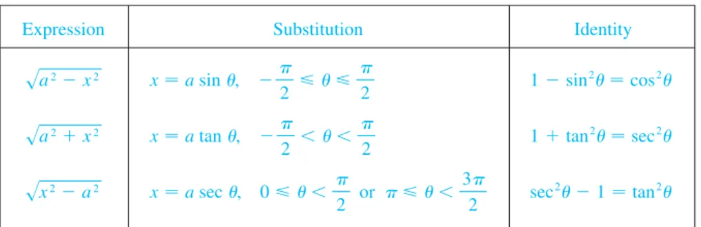
Because of the Fundamental Theorem of Calculus, we can integrate a function if we know an antiderivative, that is, an indefinite integral. We summarize here the most important integrals that we have learned so far.

In this chapter we develop techniques for using these basic integration formulas to obtain indefinite integrals of more complicated functions. We learned the most important method of integration, the Substitution Rule, in Section 5.5. The other general technique, integration by parts, is presented in Section 7.1. Then we learn methods that are special to particular classes of functions, such as trigonometric functions and rational functions.

Integration is not as straightforward as differentiation; there are no rules that absolutely guarantee obtaining an indefinite integral of a function. Therefore we discuss a strategy for integration in Section 7.5.

y

1

sa2_x2 dx苷sin

1

冉

x

a

冊

C

y

1

x2

a2 dx苷

1 a tan

1

冉

x

a

冊

C

y

cot xdx苷_ln

ⱍ

_{sin x}

ⱍ

_C

y

tan xdx苷_ln

ⱍ

_{sec x}

ⱍ

_C

y

cosh xdx苷_{sinh xC}

y

sinh xdx苷_{cosh xC}

y

csc x cot xdx苷_{csc xC}

y

sec x tan xdx苷_{sec xC}

y

csc2_{x dx苷cot xC}

y

sec2_{x dx苷tan xC}

y

cos xdx苷_{sin xC}

y

sin xdx苷_{cos xC}

y

ax

dx苷 a

x

ln aC

y

ex_dx苷ex_C

y

1

x dx苷ln

ⱍ

x

ⱍ

C 共n苷_1兲

y

xn

dx苷 x

n1

n1C

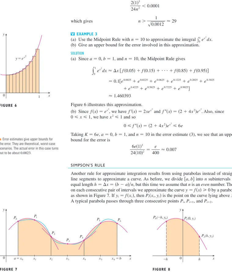
Simpson’s Rule estimates integrals by approximating graphs with parabolas.

TECHNIQUES OF

INTEGRATION

INTEGRATION BY PARTS

Every differentiation rule has a corresponding integration rule. For instance, the Substi-tution Rule for integration corresponds to the Chain Rule for differentiation. The rule that corresponds to the Product Rule for differentiation is called the rule for integration by parts.

The Product Rule states that if and are differentiable functions, then

In the notation for indefinite integrals this equation becomes

or

We can rearrange this equation as

Formula 1 is called the formula for integration by parts. It is perhaps easier to remem-ber in the following notation. Let and . Then the differentials are and , so, by the Substitution Rule, the formula for integration by parts becomes

EXAMPLE 1 Find .

SOLUTION USING FORMULA 1 Suppose we choose and . Then

and . (For we can choose anyantiderivative of .) Thus, using Formula 1, we have

It’s wise to check the answer by differentiating it. If we do so, we get , as expected.

x sin x 苷_{x cos xsin xC}

苷x cos x

y

_cos xdx 苷_{x共cos x兲}

y

_{共cos x兲dx}

y

x sin xdx苷f共x兲t共x兲

y

t共x兲f_共x兲dx t t

t共x兲苷_cos x

f_共x兲苷₁ t_共x兲苷_sin x

f共x兲苷x

y

x sin xdx

y

u dv苷uv

y

vdu

2

dv苷t共x兲dx du苷_f共x兲dx

v苷t共x兲 u苷_f共x兲

y

f共x兲t_共x兲dx苷f共x兲t共x兲

y

t共x兲f_共x兲 dx

1

y

f共x兲t_共x兲dx

y

t共_{x兲f共x兲 dx}苷_f共x兲t共_x兲

y

关f共x兲t_共x兲t共x兲f_共x兲兴dx苷f共x兲t共x兲 d

dx 关f共x兲t共x兲兴苷f共x兲t共x兲t共x兲f共x兲 t

f

7.1

SOLUTION USING FORMULA 2 Let

Then

and so

M

Our aim in using integration by parts is to obtain a simpler integral than the one we started with. Thus in Example 1 we started with and expressed it in terms

of the simpler integral . If we had instead chosen and , then

and , so integration by parts gives

Although this is true, is a more difficult integral than the one we started with. In general, when deciding on a choice for and , we usually try to choose to be a function that becomes simpler when differentiated (or at least not more complicated) as long as can be readily integrated to give .

EXAMPLE 2 Evaluate .

SOLUTION Here we don’t have much choice for and . Let

Then

Integrating by parts, we get

Integration by parts is effective in this example because the derivative of the function

is simpler than .f M

f共x兲苷_{ln x}

苷_{x ln xxC} 苷_{x ln x}

y

_dx

y

ln xdx苷x ln x

y

x dx x du苷 1

x dx v苷x u苷_ln x dv苷dx

dv u

y

ln xdx

V

v dv苷t共x兲dx

u苷f共x兲 dv

u

x

x2 cos xdx

y

x sin xdx苷_共sin x兲 x 2

2

1 2

y

x

2 cos xdx v苷x2兾2

du苷_{cos xdx}

dv苷xdx u苷_sin x

x

cos xdx

x

x sin xdx NOTE

苷x cos x_sin xC 苷x cos x

y

_cos xdx

y

x sin xdx苷

y

_{x sin xdx}苷 _{x 共cos x兲}

y

_{共cos x兲 dx} v苷cos x

du苷_dx

dv苷sin xdx u苷_x

u d√ u √ √ du

N It is helpful to use the pattern:

v苷_䊐 du苷_䊐

dv苷_䊐 u苷_䊐

NIt’s customary to write x 1 dxas x dx.

EXAMPLE 3 Find .

SOLUTION Notice that becomes simpler when differentiated (whereas is unchanged when differentiated or integrated), so we choose

Then

Integration by parts gives

The integral that we obtained, , is simpler than the original integral but is still not obvious. Therefore, we use integration by parts a second time, this time with and

. Then , , and

Putting this in Equation 3, we get

M

EXAMPLE 4 Evaluate .

SOLUTION Neither nor becomes simpler when differentiated, but we try choosing

and anyway. Then and , so integration by

parts gives

The integral that we have obtained, , is no simpler than the original one, but at least it’s no more difficult. Having had success in the preceding example integrating by parts twice, we persevere and integrate by parts again. This time we use and

. Then , , and

At first glance, it appears as if we have accomplished nothing because we have arrived at , which is where we started. However, if we put the expression for

from Equation 5 into Equation 4 we get

y

ex

sin xdx苷ex

cos xex

sin x

y

ex sin xdx

x

ex cos xdx

x

ex sin xdx

y

ex

cos xdx苷ex

sin x

y

ex sin xdx

5

v苷sin x du苷ex_dx

dv苷cos xdx

u苷ex

x

ex

cos xdx

y

ex

sin xdx苷ex

cos x

y

ex cos xdx

4

v苷cos x du苷_ex_dx

dv苷sin xdx u苷_ex

sin x ex

y

ex sin xdx

V

where C1苷2C

苷t2_et 2tet

2et_C 1

苷t2_et_2共tet_et_C兲

y

t2_et_dt苷t2_et

2

y

tet_dt

苷tet_et_C

y

tet_dt苷tet

y

_et_dt

v苷et du苷dt dv苷etdt

u苷t

x

tet_dt

y

t2_et_dt苷t2_et₂

y

_tet_dt 3

du苷_{2t dt} v苷et

u苷t2 _d

v苷etdt

et

t2

y

t2_et_dt V

SECTION 7.1 INTEGRATION BY PARTS |||| 455

This can be regarded as an equation to be solved for the unknown integral. Adding to both sides, we obtain

Dividing by 2 and adding the constant of integration, we get

M

If we combine the formula for integration by parts with Part 2 of the Fundamental Theorem of Calculus, we can evaluate definite integrals by parts. Evaluating both sides of Formula 1 between and , assuming and are continuous, and using the Fundamental Theorem, we obtain

EXAMPLE 5 Calculate .

SOLUTION Let

Then

So Formula 6 gives

To evaluate this integral we use the substitution (since has another meaning

in this example). Then , so . When , ; when ,

; so

Therefore

y

1 M

0 tan

1_xdx苷

4

y

1

0

x

1_x2 dx苷

4

ln 2 2 苷1

2共ln 2ln 1兲苷 1 2 ln 2

y

1 0

x

1_x2 dx苷 1 2

y

2

1

dt t 苷

1 2 ln

ⱍ

t

ⱍ

]

1

2

t苷₂

x苷₁ t苷₁

x苷₀ x dx苷1₂dt

dt苷₂x dx

u t苷₁x2

苷

4

y

1

0

x 1x2dx

苷_1ⴢtan1

1_0ⴢtan1 0

y

1

0

x 1x2dx

y

1 0 tan

1_{x dx苷x} tan1_x

]

0 1

y

1 0

x 1x2 dx

du苷 dx

1x2 v苷x

u苷_tan1_{x dv苷dx}

y

1 0 tan

1_{x dx}

y

b a f共x兲t

_共x兲dx苷f共x兲t共x兲

]

a b

y

b a t共x兲f

_共x兲dx

6

t f b

a

y

ex

sin xdx苷1₂ex_{共sin x}

cos x兲C 2

y

ex

sin xdx苷_ex

cos x_ex sin x

x

ex

sin xdx

N Since for , the integral in Example 5 can be interpreted as the area of the region shown in Figure 2.

x0 tan1_x0

y

0

x 1 y=tan–!x

FIGURE 2

NFigure 1 illustrates Example 4 by show-ing the graphs of and

. As a visual check on our work, notice that when has a maximum or minimum.

F f共x兲苷₀ F共x兲苷1_2ex

共sin x_{cos x兲}

f共x兲苷_ex sin x

_3

_4 12

6 F f

EXAMPLE 6 Prove the reduction formula

where is an integer.

SOLUTION Let

Then

so integration by parts gives

Since , we have

As in Example 4, we solve this equation for the desired integral by taking the last term on the right side to the left side. Thus we have

or M

The reduction formula (7) is useful because by using it repeatedly we could eventually express in terms of

x

(if is odd) or _n

x

sin x0 _dx苷

x

_dx(if is even).n

sin xdx

x

sinn_xdx

y

sinn_xdx苷1

n cos x sin

n1_x n1

n

y

sin

n2_xdx

n

y

sinn_xdx苷

cos x sinn1_xn

1

y

sinn2_xdx

y

sinn_{x dx苷}

cos x sinn1_xn

1

y

sinn2_xdxn

1

y

sinn_xdx cos2_x苷

1_sin2_x

y

sinn_xdx苷

cos x sinn1_xn

1

y

sinn2_x

cos2_xdx

v苷cos x du苷_{n1 sin}n2_x

cos xdx

dv苷sin xdx u苷_sinn1_x

n艌₂

y

sinn_{x dx苷⫺}1

ncos x sin

n⫺1_x⫹ n⫺1

n

y

sin

n⫺2_{x dx} 7

SECTION 7.1 INTEGRATION BY PARTS |||| 457

NEquation 7 is called a reduction formula because the exponent has been reduced to

and .n⫺₂ n⫺₁

n

11. 12.

13. 14.

16.

18.

19.

21. 22.

23. 24.

y

␲

0 x 3

cos xdx

y

2 1

ln x x2 dx

y

9 4

ln y

sy dy

y

1

0 t cosh tdt

y

1 0 x

2_⫹1e⫺x_dx 20.

y

␲

0 t sin 3tdt

y

e⫺␪

cos 2␪ _d␪

y

e2␪

sin 3␪ _d␪

17.

y

t sinh mtdt

y

ln x2

dx

15.

y

s 2s

ds

y

t sec2

2tdt

y

p5

ln pdp

y

arctan 4tdt 1–2 Evaluate the integral using integration by parts with the

indicated choices of and .

1. ; ,

2. ; ,

3–32 Evaluate the integral.

4.

5. 6.

7. 8.

9. 10.

y

sin⫺1

xdx

y

ln2x⫹_1dx

y

x2

cos mxdx

y

x2

sin ␲_xdx

y

t sin 2tdt

y

rer2

dr

y

xe⫺x_dx

y

x cos 5xdx

3.

dv苷cos ␪ _d␪ u苷␪

y

␪ _cos ␪ _d␪

dv苷x2dx

u苷_{ln x}

y

x2

ln xdx

dv

u

E X E R C I S E S

(b) Use part (a) to evaluate and . (c) Use part (a) to show that, for odd powers of sine,

46. Prove that, for even powers of sine,

47–50 Use integration by parts to prove the reduction formula.

48.

49.

50.

51. Use Exercise 47 to find .

52. Use Exercise 48 to find .

53–54 Find the area of the region bounded by the given curves.

53. , ,

54.

;55–56 Use a graph to find approximate -coordinates of the points of intersection of the given curves. Then find (approxi-mately) the area of the region bounded by the curves.

55. ,

56. ,

57–60 Use the method of cylindrical shells to find the volume generated by rotating the region bounded by the given curves about the specified axis.

, , ; about the -axis

58. , , ; about the -axis

59. , , , ; about

60. y苷ex, _x苷0, y苷␲; about the -axisx x苷1 x苷0

x苷⫺₁ y苷0

y苷e⫺x

y x苷₁

y苷_e⫺x

y苷_ex

y 0艋_x艋₁

y苷₀

y苷_cos␲_{x 2}

57.

y苷1_2x

y苷_{arctan 3x}

y苷_x⫺₂2

y苷_{x sin x}

x y苷_{x ln x}

y苷_{5 ln x,}

x苷5 y苷0 y苷xe⫺0.4x

x

x4

ex

dx

x

ln x3

dx

n苷1

y

secn

xdx苷 tan x sec

n⫺2

x n⫺₁

⫹ n⫺2 n⫺₁

y

sec

n⫺2

xdx n苷1 tann_xdx苷 tan

n⫺1

x n⫺₁ ⫺

y

tan

n⫺2 _xdx

y

xn

ex

dx苷_xn

ex_⫺

n

y

xn⫺1

ex

dx

y

ln xn

dx苷_{xln x}n_⫺

n

y

ln xn⫺1

dx

47.

y

␲2 0 sin

2n_xdx苷 1ⴢ3ⴢ5ⴢ ⭈ ⭈ ⭈ ⴢ2n⫺1 2ⴢ4ⴢ6ⴢ ⭈ ⭈ ⭈ ⴢ2n

␲

2

y

␲2

0 sin

2n⫹1_xdx苷 2ⴢ4ⴢ6ⴢ ⭈ ⭈ ⭈ ⴢ2n

3ⴢ5ⴢ7ⴢ ⭈ ⭈ ⭈ ⴢ2n⫹1

x

␲2

0 sin 5_xdx

x

␲2 0 sin

3_xdx

25. 26.

27. 28.

29. 30.

31. 32.

33–38 First make a substitution and then use integration by parts to evaluate the integral.

33. 34.

36.

37. 38.

;39– 42 Evaluate the indefinite integral. Illustrate, and check that your answer is reasonable, by graphing both the function and its antiderivative (take ).

39. 40.

41. 42.

43. (a) Use the reduction formula in Example 6 to show that

(b) Use part (a) and the reduction formula to evaluate .

44. (a) Prove the reduction formula

(b) Use part (a) to evaluate . (c) Use parts (a) and (b) to evaluate .

45. (a) Use the reduction formula in Example 6 to show that

where n2is an integer.

y

2

0 sin

n

xdx苷 n

₁

n

y

2 0 sin

n2

xdx

x

cos4

xdx

x

cos2

xdx

y

cosn_xdx苷 1

n cos

n1_{x sin x} n1

n

y

cos

n2_xdx

x

sin4_xdx

y

sin2_xdx苷 x

2 sin 2x

4 C

y

x2

sin 2xdx

y

x3_s

1x2 _dx

y

x32

ln xdx

y

2x3ex

dx C苷₀

y

sinln xdx

y

x ln1_xdx

y

0 e cos t

sin 2tdt

y

s

s2 3

cos2

d

35.

y

t3

et2 dt

y

cos sx dx

y

t

0e

s

sint_sds

y

2 1 x

4

ln x2

dx

y

1 0

r3

s4_r2 dr

y

cos x lnsin xdx

y

2 1

ln x2

x3 dx

y

12 0 cos

1

xdx

y

s3

1 arctan1 xdx

y

1 0

SECTION 7.1 INTEGRATION BY PARTS |||| 459

parts on the resulting integral to prove that

68. Let .

(a) Show that .

(b) Use Exercise 46 to show that

(c) Use parts (a) and (b) to show that

and deduce that .

(d) Use part (c) and Exercises 45 and 46 to show that

This formula is usually written as an infinite product:

and is called the Wallis product.

(e) We construct rectangles as follows. Start with a square of area 1 and attach rectangles of area 1 alternately beside or on top of the previous rectangle (see the figure). Find the limit of the ratios of width to height of these rectangles.

␲

2 苷 2 1 ⴢ

2 3 ⴢ

4 3 ⴢ

4 5 ⴢ

6 5ⴢ

6 7 ⴢ ⭈ ⭈ ⭈ lim

nl⬁

2 1 ⴢ

2 3 ⴢ

4 3ⴢ

4 5 ⴢ

6 5 ⴢ

6 7 ⴢ ⭈ ⭈ ⭈ ⴢ

2n 2n⫺1 ⴢ

2n 2n⫹1 苷

␲

2 limnl⬁I2n⫹1 I2n苷1

2n⫹₁ 2n⫹₂ 艋

I2n⫹1

I2n

艋₁ I2n⫹2

I2n

苷 2n

⫹₁ 2n⫹₂ I2n⫹2艋I2n⫹1艋I2n

In苷

x

␲2 0 sin

n

xdx

y

0 a b x

c d

x=a

x=b y=ƒ x=g(y)

V苷

y

b

a 2

␲_{x fxdx} 61. Find the average value of on the interval .

62. A rocket accelerates by burning its onboard fuel, so its mass decreases with time. Suppose the initial mass of the rocket at liftoff (including its fuel) is , the fuel is consumed at rate , and the exhaust gases are ejected with constant velocity (relative to the rocket). A model for the velocity of the rocket at time is given by the equation

where is the acceleration due to gravity and is not too

large. If , kg, kg s, and

, find the height of the rocket one minute after liftoff.

A particle that moves along a straight line has velocity meters per second after seconds. How far will it travel during the first seconds?

64. If and and are continuous, show that

65. Suppose that , , , , and

is continuous. Find the value of .

(a) Use integration by parts to show that

(b) If and are inverse functions and is continuous, prove that

[Hint:Use part (a) and make the substitution .] (c) In the case where and are positive functions and

, draw a diagram to give a geometric interpre-tation of part (b).

(d) Use part (b) to evaluate .

67. We arrived at Formula 6.3.2, , by using cylindrical shells, but now we can use integration by parts to prove it using the slicing method of Section 6.2, at least for the case where is one-to-one and therefore has an inverse function . Use the figure to show that

Make the substitution y苷fxand then use integration by V苷␲_b2_d⫺␲a2_c⫺

y

d

c

␲t_y2 _dy

t f

V苷

x

b

a 2␲x fxdx

x

e

1 ln xdx

b⬎_a⬎₀

t f

y苷_fx

y

b a fxdx

苷bfb⫺afa⫺

y

fb

fa tydy

f t

f

y

fxdx苷_{x fx}

y

_{x fxdx}

66.

x

4

1x fxdx

f

f4苷3 f1苷5

f4苷7 f1苷2

y

a

0 fxt

_xdx苷_fat_afata

y

a 0 f

xt_xdx t

f f0苷t₀苷₀

t

t

vt苷t2

et 63.

v_e苷3000 ms

r苷₁₆₀

m苷_30,000

t苷_{9.8 ms}2

t t

vt苷ttv_eln m

_rt m t

v_e

r m

1, 3 fx苷x2

TRIGONOMETRIC INTEGRALS

In this section we use trigonometric identities to integrate certain combinations of trigo-nometric functions. We start with powers of sine and cosine.

EXAMPLE 1 Evaluate .

SOLUTION Simply substituting isn’t helpful, since then . In order to integrate powers of cosine, we would need an extra factor. Similarly, a power of sine would require an extra factor. Thus here we can separate one cosine factor and convert the remaining factor to an expression involving sine using the identity

:

We can then evaluate the integral by substituting , so and

M

In general, we try to write an integrand involving powers of sine and cosine in a form where we have only one sine factor (and the remainder of the expression in terms of cosine) or only one cosine factor (and the remainder of the expression in terms of sine). The identity enables us to convert back and forth between even powers of sine and cosine.

EXAMPLE 2 Find .

SOLUTION We could convert to , but we would be left with an expression in terms of with no extra factor. Instead, we separate a single sine factor and rewrite the remaining factor in terms of :

Substituting , we have and so

M 苷⫺1

3cos 3_x⫹2

5cos 5_x⫺1

7cos 7_x⫹C

苷⫺

冉

u 3

3 ⫺2 u5

5 ⫹

u7 7

冊

⫹C 苷

y

_共1⫺_u2_兲2_u2_{共⫺du兲苷⫺}

y

_共u2_⫺

2u4_⫹u6_兲du

苷

y

_共1⫺_cos2x兲2 cos2_x

sin xdx

y

sin5_x

cos2_xdx苷

y

_共sin2_x兲2 cos2_x

sin xdx du苷⫺_{sin xdx} u苷_{cos x}

sin5_x

cos2_x苷共sin2_x兲2 cos2_x

sin x苷_共1⫺_cos2_x兲2 cos2_x

sin x cos x

sin4_x cos x sin x

1⫺_sin2_x cos2_x

y

sin5_x

cos2_xdx V

sin2_x⫹

cos2_x苷 1 苷_{sin x}⫺1

3 sin 3_x⫹C

苷

y

_共1⫺_u2_兲du苷u⫺1 3u

3_⫹C

y

cos3_xdx苷

y

cos2_x

ⴢcos xdx苷

y

共1⫺sin2x兲 cos xdx

du苷_cos xdx u苷_sin x

cos3_x苷 cos2_x

ⴢcos x苷共1⫺sin2x兲 cos x sin2_x⫹

cos2_x苷 1

cos2_x cos x

sin x

du苷⫺_{sin xdx} u苷_cos x

y

cos3_xdx

7.2

N Figure 1 shows the graphs of the integrand in Example 2 and its indefinite inte-gral (with C苷₀). Which is which?

sin5_{x cos}2_x

FIGURE 1

_π

_0.2 0.2

In the preceding examples, an odd power of sine or cosine enabled us to separate a single factor and convert the remaining even power. If the integrand contains even powers of both sine and cosine, this strategy fails. In this case, we can take advantage of the fol-lowing half-angle identities (see Equations 17b and 17a in Appendix D):

and

EXAMPLE 3 Evaluate .

SOLUTION If we write , the integral is no simpler to evaluate. Using the half-angle formula for , however, we have

Notice that we mentally made the substitution when integrating . Another method for evaluating this integral was given in Exercise 43 in Section 7.1. M

EXAMPLE 4 Find .

SOLUTION We could evaluate this integral using the reduction formula for

(Equation 7.1.7) together with Example 3 (as in Exercise 43 in Section 7.1), but a better method is to write and use a half-angle formula:

Since occurs, we must use another half-angle formula

This gives

M

To summarize, we list guidelines to follow when evaluating integrals of the form , where and are _m0 n₀ integers.

x

sinm_x

cosn_xdx

苷1₄

(

3₂x_{sin 2}x1_{8 sin 4}x

)

C 苷1₄

y

(

3_{22 cos 2}x1_{2 cos 4}x

)

dx

y

sin4_xdx苷1

4

y

12 cos 2x 1

21cos 4xdx cos2

2x苷1

21cos 4x cos2

2x

苷1₄

y

_{12 cos 2}x_cos2 2xdx 苷

y

冉

1cos 2x

2

冊

2

dx

y

sin4_xdx苷

y

_共sin2_x兲2 _dx sin4_x苷共sin2_x兲2

x

sinn_xdx

y

sin4_xdx

cos 2x u苷₂x

苷1

2

(

1

2 sin 2

)

1 2

(

0

1

2 sin 0

)

苷 1 2

y

0 sin

2_xdx苷1 2

y

0 共1

_{cos 2x兲 dx}苷

[

1

2

(

x 1

2 sin 2x

)

]

0

sin2_x sin2_x苷

1_cos2_x

y

0 sin 2_xdx V

cos2_x苷1

2共1cos 2x兲 sin2_x苷1

2共1cos 2x兲

SECTION 7.2 TRIGONOMETRIC INTEGRALS |||| 461

NExample 3 shows that the area of the region shown in Figure 2 is _兾2.

FIGURE 2

0

_0.5 1.5

STRATEGY FOR EVALUATING

(a) If the power of cosine is odd , save one cosine factor and use to express the remaining factors in terms of sine:

Then substitute .

(b) If the power of sine is odd , save one sine factor and use to express the remaining factors in terms of cosine:

Then substitute . [Note that if the powers of both sine and cosine are odd, either (a) or (b) can be used.]

(c) If the powers of both sine and cosine are even, use the half-angle identities

It is sometimes helpful to use the identity

We can use a similar strategy to evaluate integrals of the form . Since , we can separate a factor and convert the remaining (even) power of secant to an expression involving tangent using the identity .

Or, since , we can separate a factor and convert the

remaining (even) power of tangent to secant.

EXAMPLE 5 Evaluate .

SOLUTION If we separate one factor, we can express the remaining factor in terms of tangent using the identity . We can then evaluate the integral

by substituting so that :

M 苷1

7 tan 7_x⫹1

9 tan 9_x⫹C

苷 u

7

7 ⫹

u9

9 ⫹C

苷

y

_u6

1⫹u2_du苷

y

_u6_⫹u8_du

苷

y

_tan6_x

1⫹tan2_x

sec2_xdx

y

tan6_x

sec4_xdx苷

y

tan6_x

sec2_x

sec2_xdx

du苷_sec2xdx u苷_tan x

sec2_x苷

1⫹tan2_x

sec2_x sec2_x

y

tan6_x

sec4_xdx V

sec x tan x

ddx sec x苷_{sec x tan x}

sec2_x苷

1⫹tan2_x sec2_x

ddx tan x苷_sec2_x

x

tanm_x

secn_xdx sin x cos x苷1_{2sin 2}x

cos2_x苷1

21⫹cos 2x sin2_x苷1

21⫺cos 2x

u苷_{cos x}

苷

y

_1⫺cos2_xk cosn_x

sin xdx

y

sin2k⫹1_x

cosn_xdx苷

y

sin2_xk

cosn_x

sin xdx sin2_x苷

1⫺cos2_x

m苷₂k⫹1

u苷_sin x

苷

y

_sinm_x1⫺sin2_xk cos xdx

y

sinm_x

cos2k⫹1_xdx苷

y

sinm_x

cos2_xk cos xdx cos2_x苷

1⫺sin2_x

n苷_2k⫹1

EXAMPLE 6 Find .

SOLUTION If we separate a factor, as in the preceding example, we are left with a factor, which isn’t easily converted to tangent. However, if we separate a

factor, we can convert the remaining power of tangent to an expression involving only secant using the identity . We can then evaluate the

integral by substituting , so :

M

The preceding examples demonstrate strategies for evaluating integrals of the form for two cases, which we summarize here.

STRATEGY FOR EVALUATING

(a) If the power of secant is even , save a factor of and use to express the remaining factors in terms of :

Then substitute .

(b) If the power of tangent is odd , save a factor of and

use to express the remaining factors in terms of :

Then substitute .

For other cases, the guidelines are not as clear-cut. We may need to use identities, inte-gration by parts, and occasionally a little ingenuity. We will sometimes need to be able to

u苷_{sec x}

苷

y

_sec2_x⫺ 1k

secn⫺1_x

sec x tan xdx

y

tan2k⫹1_x

secn_xdx苷

y

tan2_xk

secn⫺1_x

sec x tan xdx

sec x tan2_x苷

sec2_x

⫺1

sec x tan x

m苷₂k⫹1

u苷_tan x

苷

y

_tanm_x1⫹tan2_xk⫺1 _sec2_xdx

y

tanm_x

sec2k_xdx苷

y

tanm_x

sec2_xk⫺1 sec2_xdx

tan x sec2_x苷

1⫹tan2_x

sec2_x

n苷_{2k, k艌2}

y

tanm_{x sec}n_{x dx}

x

tanm_x

secn_xdx

苷₁₁1 _sec11_{␪ ⫺}2_{9 sec}9_{␪ ⫹}1_{7 sec}7_{␪ ⫹}C

苷 u

11

11 ⫺2 u9

9 ⫹

u7

7 ⫹C

苷

y

_u10_⫺

2u8_⫹u6_du

苷

y

_u2_⫺

12_u6 _du

苷

y

_sec2_{␪ ⫺} 12

sec6_␪

sec ␪ tan ␪d␪

y

tan5_␪

sec7_␪d␪苷

y

tan4_␪

sec6_␪

sec ␪ tan ␪d␪

du苷_{sec ␪ tan ␪d␪} u苷_{sec ␪}

tan2_␪苷sec2_{␪ ⫺1} sec ␪ tan ␪

sec5_␪

sec2_␪

y

tan5_␪

sec7_␪d␪

integrate by using the formula established in (5.5.5):

We will also need the indefinite integral of secant:

We could verify Formula 1 by differentiating the right side, or as follows. First we

multi-ply numerator and denominator by :

If we substitute , then , so the integral

becomes . Thus we have

EXAMPLE 7 Find .

SOLUTION Here only occurs, so we use to rewrite a factor in

terms of :

In the first integral we mentally substituted so that . M

If an even power of tangent appears with an odd power of secant, it is helpful to express the integrand completely in terms of . Powers of may require integration by parts, as shown in the following example.

EXAMPLE 8 Find .

SOLUTION Here we integrate by parts with

du苷_sec x tan xdx v苷tan x u苷_{sec x d}v苷sec2xdx

y

sec3_xdx

sec x sec x

du苷_sec2xdx u苷_tan x

苷 tan

2_x

2 ⫺ln

ⱍ

sec x

ⱍ

⫹C 苷

y

_tan x sec2_xdx

⫺

y

tan xdx 苷

y

_{tan x共sec}2_x⫺

1兲dx

y

tan3_xdx苷

y

tan x tan2_xdx sec2_x

tan2_x tan2_x苷

sec2_x

⫺1 tan x

y

tan3_xdx

y

sec xdx苷_ln

ⱍ

_{sec x⫹tan x}

ⱍ

_⫹C

x

共1兾u兲du苷_ln

ⱍ

_u

ⱍ

_⫹C

du苷_{共sec x tan x⫹sec}2_x

兲dx u苷_{sec x⫹tan x}

苷

y

sec

2_x

⫹sec x tan x sec x⫹tan x dx

y

sec xdx苷

y

_{sec x} sec x⫹tan x sec x⫹tan x dx sec x⫹tan x

y

sec xdx苷_ln

ⱍ

_{sec x⫹tan x}

ⱍ

_⫹C

1

Then

Using Formula 1 and solving for the required integral, we get

M

Integrals such as the one in the preceding example may seem very special but they occur frequently in applications of integration, as we will see in Chapter 8. Integrals of the form can be found by similar methods because of the identity

.

Finally, we can make use of another set of trigonometric identities:

To evaluate the integrals (a) , (b) , or

(c) , use the corresponding identity:

(a)

(b)

(c)

EXAMPLE 9 Evaluate .

SOLUTION This integral could be evaluated using integration by parts, but it’s easier to use the identity in Equation 2(a) as follows:

M 苷1₂

(

_cos x⫺19cos 9x⫹C

苷1

2

y

⫺sin x⫹sin 9xdx

y

sin 4x cos 5xdx苷

y

1

2关sin共⫺x兲⫹sin 9x兴dx

y

sin 4x cos 5xdx cos A cos B苷1

2关cos共A⫺B兲⫹cos共A⫹B兲兴 sin A sin B苷1

2关cos共A⫺B兲⫺cos共A⫹B兲兴 sin A cos B苷1

2关sin共A⫺B兲⫹sin共A⫹B兲兴

x

cos mx cos nxdx

x

sin mx sin nxdx

x

sin mx cos nxdx

2 1⫹cot2_x苷

csc2_x

x

cotm_x

cscn_xdx

y

sec3_xdx苷1

2

(

sec x tan x⫹ln

ⱍ

sec x⫹tan x

ⱍ

)

⫹C

苷_sec x tan x⫺

y

sec3_xdx

⫹

y

sec xdx 苷_sec x tan x⫺

y

sec x共sec2_x

⫺1兲dx

y

sec3_xdx苷

sec x tan x⫺

y

sec x tan2_xdx

SECTION 7.2 TRIGONOMETRIC INTEGRALS |||| 465

NThese product identities are discussed in Appendix D.

9. 10.

11. 12.

14.

15. 16.

y

cos ␪ cos5

共sin ␪兲d␪

y

cos5_␣

ssin ␣ d␣

y

␲

0 sin 2

t cos4

tdt

y

␲兾2 0 sin

2

x cos2

xdx

13.

y

x cos2_xdx

y

共1⫹cos ␪兲2_d␪

y

␲

0 cos 6_␪

d␪

y

␲

0 sin 4

共3t兲dt 1– 49 Evaluate the integral.

1. 2.

4.

5. 6.

8.

y

␲兾2

0 sin 2

共2␪兲d␪

y

␲兾2 0 cos

2_␪

d␪

7.

y

sin3

(

_sx

)

sx dx

y

sin2

共␲x兲 cos5

共␲x兲dx

y

␲兾2 0 cos

5

xdx

y

3␲兾4

␲兾2 sin 5

x cos3

xdx

3.

y

sin6_{x cos}3_xdx

y

sin3_{x cos}2_xdx E X E R C I S E S

53. 54.

Find the average value of the function on the interval .

56. Evaluate by four methods: (a) the substitution

(b) the substitution (c) the identity (d) integration by parts

Explain the different appearances of the answers.

57–58 Find the area of the region bounded by the given curves.

57.

58. , ,

;59–60 Use a graph of the integrand to guess the value of the integral. Then use the methods of this section to prove that your guess is correct.

59. 60.

61–64 Find the volume obtained by rotating the region bounded by the given curves about the specified axis.

, , ; about the -axis

62. , , ; about the -axis

63. , , ; about

64. , , ; about

65. A particle moves on a straight line with velocity function . Find its position function

if

66. Household electricity is supplied in the form of alternating current that varies from V to V with a frequency of 60 cycles per second (Hz). The voltage is thus given by the equation

where is the time in seconds. Voltmeters read the RMS (root-mean-square) voltage, which is the square root of the average value of over one cycle.

(a) Calculate the RMS voltage of household current. (b) Many electric stoves require an RMS voltage of 220 V.

Find the corresponding amplitude needed for the volt-age .Et苷A sin120␲_t

A 关E共t兲兴2

t

E共t兲苷155 sin共120␲_t兲

⫺155 155

f共0兲苷_0.

s苷_f共t兲

v共t兲苷sin ␻t cos2␻t

y苷_⫺1

0艋x艋␲兾3 y苷_{cos x}

y苷_{sec x}

y苷₁

0艋x艋␲兾4 y苷_{cos x}

y苷_{sin x}

x 0艋x艋␲

y苷₀

y苷_sin2

x

x

␲兾2艋x艋␲

y苷₀

y苷_{sin x}

61.

y

2

0 sin 2␲x cos 5␲xdx

y

2␲

0 cos 3

xdx

␲兾4艋x艋5␲兾4 y苷_cos3

x y苷_sin3

x

⫺␲兾4艋x艋␲兾4 y苷cos2

x, y苷sin2

x,

sin 2x苷2 sin x cos x u苷_{sin x}

u苷cos x

x

sin x cos xdx

关⫺␲, ␲兴

f共x兲苷_sin2

x cos3

x

55.

y

sec4 x

2dx

y

sin 3x sin 6xdx

17. 18. 19. 20. 21. 22. 24. 25. 26. 27. 28. 30. 31. 32. 33. 34. 35. 36. 37. 38. 39. 40. 41. 42. 44. 45. 46. 47. 48. 49.

50. If , express the value of

in terms of .

;51–54 Evaluate the indefinite integral. Illustrate, and check that your answer is reasonable, by graphing both the integrand and its antiderivative (taking .

51. 52.

y

sin3

x cos4

xdx

y

x sin2

共x2

兲dx

C苷_0兲

I

x

␲兾4

0 tan 8

x sec xdx

x

␲兾4

0 tan 6

x sec xdx苷_I

y

t sec2

共t2

兲 tan4

共t2

兲dt

y

dx cos x⫺1

y

1⫺tan2_x

sec2_x dx

y

cos x⫹sin x sin 2x dx

y

sin 5␪ sin ␪ d␪

y

cos ␲x cos 4␲xdx

y

sin 8x cos 5xdx

43.

y

␲兾3

␲兾6 csc 3

xdx

y

csc xdx

y

csc4

x cot6

xdx

y

cot3

␣ csc3

␣ d␣

y

␲兾2

␲兾4 cot 3_xdx

y

␲兾2

␲兾6 cot 2_xdx

y

sin ␾

cos3_␾ d␾

y

x sec x tan xdx

y

tan2

x sec xdx

y

tan3_␪

cos4_␪ d␪

y

tan6_共ay兲dy

y

tan5_xdx

y

␲兾3 0 tan

5

x sec6

xdx

y

tan3

x sec xdx

29.

y

tan3

共2x兲 sec5

共2x兲dx

y

␲兾3 0 tan

5

x sec4

xdx

y

␲兾4 0 sec

4_␪

tan4_␪

d␪

y

sec6

tdt

y

共tan2

x⫹tan4

x兲dx

y

tan2

xdx

23.

y

␲兾2 0 sec

4

共t兾2兲dt

y

sec2

x tan xdx

y

cos2

x sin 2xdx

y

cos x⫹sin 2x sin x dx

y

cot5

␪ sin4

␪d␪

y

cos2

x tan3

SECTION 7.3 TRIGONOMETRIC SUBSTITUTION |||| 467

70. A finite Fourier series is given by the sum

Show that the th coefficient is given by the formula

am苷 1 ␲

y

␲

⫺␲ fxsin mxdx am

m

苷_{a1sin x⫹a2sin 2x⫹ ⭈ ⭈ ⭈ ⫹aNsin Nx}

fx苷

兺

N

n苷1

ansin nx 67–69 Prove the formula, where and are positive integers.

67.

68.

69.

y

␲

⫺␲ cos mx cos nxdx

苷

再

0

␲

if m苷_n

if m苷n

y

␲

⫺␲ sin mx sin nxdx

苷

再

0

␲

if m苷_n

if m苷_n

y

␲

⫺␲ sin mx cos nxdx

苷0

n m

TRIGONOMETRIC SUBSTITUTION

In finding the area of a circle or an ellipse, an integral of the form arises,

where . If it were , the substitution would be effective

but, as it stands, is more difficult. If we change the variable from to by the substitution , then the identity allows us to get rid of the root sign because

Notice the difference between the substitution (in which the new variable is a function of the old one) and the substitution (the old variable is a function of the new one).

In general we can make a substitution of the form by using the Substitution Rule in reverse. To make our calculations simpler, we assume that has an inverse func-tion; that is, is one-to-one. In this case, if we replace by and by in the Substitution Rule (Equation 5.5.4), we obtain

This kind of substitution is called inverse substitution.

We can make the inverse substitution provided that it defines a one-to-one function. This can be accomplished by restricting to lie in the interval .

In the following table we list trigonometric substitutions that are effective for the given radical expressions because of the specified trigonometric identities. In each case the restric-tion on is imposed to ensure that the funcrestric-tion that defines the substiturestric-tion is one-to-one. (These are the same intervals used in Section 1.6 in defining the inverse functions.)

TABLE OF TRIGONOMETRIC SUBSTITUTIONS

␪

关⫺␲兾2, ␲兾2兴

␪

x苷_{a sin ␪}

y

f共x兲dx苷

y

f共t共t兲兲t⬘共t兲dt

t x x u

t t

x苷t_共t兲

x苷a sin ␪

u苷a2

⫺x2

sa2_⫺x2 _苷s_a2_⫺a2_sin2_{␪ 苷}s_a2_共1⫺sin2_{␪兲 苷}s_a2_cos2_{␪ 苷a}

ⱍ

cos ␪

ⱍ

1⫺sin2_␪苷 cos2_␪

x苷_{a sin ␪}

␪

x

x

sa2_⫺x2 _dx

u苷a2

⫺x2

x

xsa2_⫺x2 _dx

a⬎0

x

sa2_⫺x2 _dx

7.3

Expression Substitution Identity

sec2

␪ ⫺1苷tan2 ␪

x苷a sec ␪, 0艋␪ ⬍ ␲

2 or ␲ 艋 ␪ ⬍ 3␲

2

sx2_⫺a2

1⫹tan2_␪苷sec2_␪

x苷a tan ␪, ⫺␲

2 ⬍ ␪ ⬍

␲

2

sa2_⫹x2

1⫺sin2_␪苷

cos2_␪

x苷_{a sin ␪, ⫺}␲

2 艋␪ 艋

␲

2

EXAMPLE 1 Evaluate .

SOLUTION Let , where . Then and

(Note that because .) Thus the Inverse Substitution Rule

gives

Since this is an indefinite integral, we must return to the original variable . This can be done either by using trigonometric identities to express in terms of or by drawing a diagram, as in Figure 1, where is interpreted as an angle of a right tri-angle. Since , we label the opposite side and the hypotenuse as having lengths and . Then the Pythagorean Theorem gives the length of the adjacent side as , so we can simply read the value of from the figure:

(Although in the diagram, this expression for is valid even when .)

Since , we have and so

M

EXAMPLE 2 Find the area enclosed by the ellipse

SOLUTION Solving the equation of the ellipse for , we get

Because the ellipse is symmetric with respect to both axes, the total area is four times the area in the first quadrant (see Figure 2). The part of the ellipse in the first quadrant is given by the function

and so 14A苷

y

a

0

b a sa

2_⫺x2 _dx 0艋 x艋a y苷 b

a sa

2_⫺x2

A y苷_⫾b

a sa

2_⫺x2 or

y2

b2 苷1⫺

x2

a2 苷

a2_⫺x2

a2

y x2

a2 ⫹

y2

b2 苷1 V

y

s9⫺x2

x2 dx苷⫺

s9⫺x2

x ⫺sin

⫺1

x 3

⫹C

␪苷_sin⫺1_x 3

sin ␪苷_x3

␪ ⬍0 cot ␪

␪ ⬎0

cot ␪苷 s9⫺x

2

x cot ␪

s9⫺x2 3

x sin ␪苷_x3

␪

sin ␪苷_x3 cot ␪

x 苷_{⫺cot ␪ ⫺ ␪ ⫹}C

苷

y

_csc2_{␪ ⫺} 1d␪

苷

y

cos

2

␪

sin2

␪ d␪苷

y

cot

2_{␪ d␪}

y

s9⫺x2

x2 dx苷

y

3 cos ␪

9 sin2_␪ 3 cos ␪ d␪

⫺␲2艋␪ 艋 ␲2 cos ␪ 艌0

s9⫺x2 _苷s9_{⫺9 sin}2_{␪ 苷}s9 cos2_{␪ 苷3}

ⱍ

_{cos ␪}

ⱍ

_{苷3 cos ␪}

dx苷_{3 cos ␪ d␪}

⫺␲兾2艋␪ 艋 ␲兾2 x苷_{3 sin ␪}

y

s9⫺x2

x2 dx V

3

¨

x

œ„„„„„9-≈

FIGURE 1

sin¨=x

3

FIGURE 2

≈ a@

¥ b@

+ =1

y

0 x

(0, b)

To evaluate this integral we substitute . Then . To change the limits of integration we note that when , , so ; when ,

, so . Also

since . Therefore

We have shown that the area of an ellipse with semiaxes and is . In particular, taking , we have proved the famous formula that the area of a circle with

radius is . M

Since the integral in Example 2 was a definite integral, we changed the limits of integration and did not have to convert back to the original variable .

EXAMPLE 3 Find .

SOLUTION Let . Then and

Thus we have

To evaluate this trigonometric integral we put everything in terms of and :

Therefore, making the substitution , we have

We use Figure 3 to determine that and so

M

y

dx

x2_sx2_⫹4 苷⫺

sx2_⫹4

4x ⫹C

csc ␪苷s_x2_⫹4x

苷_⫺csc ␪

4 ⫹C

苷 1

4

⫺ 1

u

⫹C苷⫺ 1 4 sin ␪ ⫹C

y

dx

x2_sx2_⫹4 苷 1 4

y

cos ␪

sin2

␪ d␪苷

1 4

y

du u2

u苷_{sin ␪} sec ␪

tan2

␪ 苷

1 cos ␪ ⴢ

cos2

␪

sin2

␪ 苷

cos ␪

sin2

␪

cos ␪

sin ␪

y

dx

x2s_x2_⫹4 苷

y

2 sec2_{␪ d␪} 4 tan2_␪

ⴢ2 sec ␪

苷 1

4

y

sec ␪

tan2_␪ d␪ sx2_{⫹4 苷}s4_tan2_{␪ ⫹1 苷}s4 sec2_{␪ 苷2}

ⱍ

_{sec ␪}

ⱍ

_{苷2 sec ␪}

dx苷_{2 sec}2_{␪ d␪}

x苷_{2 tan ␪, ⫺␲兾2⬍ ␪ ⬍ ␲兾2}

y

1

x2s_x2_⫹4 dx V

x NOTE

␲r2

r

a苷_b苷_r

␲ab b a 苷₂ab

[

␪ ⫹12sin 2␪

]

0

␲兾2

苷 ₂ab

冉

␲

2 ⫹0⫺0

冊

苷␲ab 苷_4ab

y

␲兾2

0 cos 2_{␪ d␪苷}

4ab

y

␲兾2

0 1

2共1⫹cos 2␪兲d␪

A苷₄ b a

y

a

0 sa

2_⫺x2 _dx苷4 b

a

y

␲兾2

0 a cos ␪ⴢa cos ␪ d␪ 0艋␪ 艋 ␲兾2

sa2_⫺x2 _苷s_a2_⫺a2_sin2_{␪ 苷}s_a2_cos2_{␪ 苷a}

ⱍ

_{cos ␪}

ⱍ

_{苷a cos ␪}

␪苷_␲兾2 sin ␪苷₁

x苷_a

␪苷₀ sin ␪苷₀

x苷₀

dx苷_{a cos ␪ d␪} x苷_{a sin ␪}

SECTION 7.3 TRIGONOMETRIC SUBSTITUTION |||| 469

œ„„„„„≈+4

2 ¨

x

FIGURE 3

tan¨=x

EXAMPLE 4 Find .

SOLUTION It would be possible to use the trigonometric substitution here (as in Example 3). But the direct substitution is simpler, because then

and

M

Example 4 illustrates the fact that even when trigonometric substitutions are possible, they may not give the easiest solution. You should look for a simpler method first.

EXAMPLE 5 Evaluate , where .

SOLUTION 1 We let , where or . Then

and

Therefore

The triangle in Figure 4 gives , so we have

Writing , we have

SOLUTION 2 For the hyperbolic substitution can also be used. Using the

identity , we have

Since , we obtain

Since , we have and

y

dx

sx2_⫺a2 苷cosh

⫺1

x

a

⫹C

2

t苷_cosh⫺1_xa cosh t苷_xa

y

dx

sx2_⫺a2 苷

y

a sinh tdt

a sinh t 苷

y

dt苷t⫹C dx苷_{asinh tdt}

sx2_⫺a2 苷s_a2_cosh2_t⫺1 苷s_a2_sinh2_t 苷_{a sinh t} cosh2_y⫺sinh2_y苷1

x苷_{acosh t} x⬎0

y

dx

sx2_⫺a2 苷ln

ⱍ

x⫹sx

2_⫺a2

ⱍ

_⫹C 1 1

C1苷C⫺ln a

苷_ln

ⱍ

_x⫹s_x2_⫺a2

ⱍ

_{⫺ln a⫹C}

y

dx

sx2_⫺a2 苷ln

冟

x a ⫹

sx2_⫺a2

a

冟

⫹C tan ␪苷s_x2_⫺a2 _兾a

苷

y

_{sec ␪ d␪}苷_ln

ⱍ

_{sec ␪ ⫹tan ␪}

ⱍ

_⫹C

y

dx

sx2_⫺a2 苷

y

a sec ␪ tan ␪

a tan ␪ d␪

sx2_⫺a2 苷s_a2_共sec2_{␪ ⫺1兲} 苷s_a2_tan2_␪ 苷_a

ⱍ

_{tan ␪}

ⱍ

苷_{a tan ␪} dx苷_{a sec ␪ tan ␪ d␪}

␲ ⬍ ␪ ⬍3␲兾2 0⬍ ␪ ⬍ ␲兾2

x苷_{a sec ␪}

a⬎0

y

dx

sx2_⫺a2

NOTE

y

x

sx2_⫹4 dx苷 1 2

y

du

su 苷su ⫹C苷sx

2_{⫹4 ⫹C}

du苷_2xdx u苷_x2_⫹

4

x苷_{2 tan ␪}

y

x

sx2_⫹4 dx

FIGURE 4

sec¨=x a

œ„„„„„

a ¨

x

Although Formulas 1 and 2 look quite different, they are actually equivalent by

Formula 3.11.4. M

As Example 5 illustrates, hyperbolic substitutions can be used in place of trigo-nometric substitutions and sometimes they lead to simpler answers. But we usually use trigonometric substitutions because trigonometric identities are more familiar than hyper-bolic identities.

EXAMPLE 6 Find .

SOLUTION First we note that so trigonometric substitution

is appropriate. Although is not quite one of the expressions in the table of trigonometric substitutions, it becomes one of them if we make the preliminary substitu-tion . When we combine this with the tangent substitution, we have ,

which gives and

When , , so ; when , , so .

Now we substitute so that . When , ; when

. Therefore

M

EXAMPLE 7 Evaluate .

SOLUTION We can transform the integrand into a function for which trigonometric substitu-tion is appropriate by first completing