Table of Contents
Beginning Application Development with TensorFlow and Keras Why subscribe?
1. Introduction to Neural Networks and Deep Learning Lesson Objectives
What are Neural Networks? Successful Applications
Why Do Neural Networks Work So Well? Representation Learning
Function Approximation Limitations of Deep Learning
Inherent Bias and Ethical Considerations
Activity 1 – Verifying Software Components Activity 2 – Exploring a Trained Neural Network
Summary
Activity 3 – Exploring the Bitcoin Dataset and Preparing Data for Model Using Keras as a TensorFlow Interface
Model Components
Activity 4 – Creating a TensorFlow Model Using Keras From Data Preparation to Modeling
Training a Neural Network
Reshaping Time-Series Data Making Predictions
Overfitting
Interpreting Predictions
Activity 6 – Creating an Active Training Environment Hyperparameter Optimization
Layers and Nodes - Adding More Layers Adding More Nodes
Activity 7 – Optimizing a Deep Learning Model Summary
Activity 8 – Dealing with New Data
Deploying a Model as a Web Application Application Architecture and Technologies
Deploying and Using Cryptonic
Activity 9 – Deploying a Deep Learning Application Summary
Beginning Application Development with
TensorFlow and Keras
Copyright © 2018 Packt Publishing
All rights reserved. No part of this book may be reproduced, stored in a retrieval system, or transmitted in any form or by any means, without the prior written permission of the publisher, except in the case of brief quotations embedded in critical articles or reviews.
Every effort has been made in the preparation of this book to ensure the accuracy of the information presented. However, the information contained in this book is sold without warranty, either express or implied. Neither the author, nor Packt Publishing, and its dealers and distributors will be held liable for any damages caused or alleged to be caused directly or indirectly by this book.
Packt Publishing has endeavored to provide trademark information about all of the companies and products mentioned in this book by the appropriate use of capitals. However, Packt Publishing cannot guarantee the accuracy of this information.
Acquisition Editor: Koushik Sen
Development Editor: Tanmayee Patil
Production Coordinator: Vishal Pawar, Samita Warang
First published: April 2018
Production reference: 1300418
Published by Packt Publishing Ltd.
Livery Place
35 Livery Street
Birmingham B3 2PB, UK.
ISBN 978-1-78953-729-1
https://mapt.packtpub.com/
Mapt is an online digital library that gives you full access to over 5,000 books and videos, as well as industry leading tools to help you plan your personal development and advance your career. For more information, please visit https://mapt.packtpub.com/ website.
Why subscribe?
Spend less time learning and more time coding with practical eBooks and Videos from over 4,000 industry professionals
Improve your learning with Skill Plans built especially for you Get a free eBook or video every month
Mapt is fully searchable
PacktPub.com
Did you know that Packt offers eBook versions of every book published, with PDF and ePub files available? You can upgrade to the eBook version at www.PacktPub.com and as a print book customer, you are entitled to a discount on the eBook copy. Get in touch with us at <[email protected]> for more details.
Contributors
About the author
Luis Capelo is a Harvard-trained analyst and programmer who specializes in the design and development of data science products. He is based in the great New York City, USA.
He is the head of the Data Products team at Forbes, where they both investigate new techniques for optimizing article performance and create clever bots that help them distribute their content. Previously, he led a team of world-class scientists at the Flowminder Foundation, where we developed predictive models for assisting the humanitarian community. Prior to that, he worked for the United Nations as part of the Humanitarian Data Exchange team (founders of the Center for Humanitarian Data).
About the reviewer
Preface
TensorFlow is one of the most popular architectures used for machine learning and, more recently, deep learning. This book is your guide to deploy TensorFlow and Keras models into real-world applications.
The book begins with a dedicated blueprint for how to build an application that generates predictions. Each subsequent lesson tackles a particular type of model, such as neural networks, configuring a deep learning environment, using Keras and focuses on the three important questions of how the model works, how to improve our prediction accuracy in our example model, and how to measure and assess its performance using real-world applications.
In this book, you will learn how to create an application that generates predictions from deep learning. This learning journey begins by exploring the common components of a neural network and its essential performance. By end of the lesson you will be exploring a trained neural network created using TensorFlow. In the remaining lessons, you will learn to build a deep learning model with different components together and measuring their performance in prediction. Finally, we will be able to deploy a working web-application
What This Book Covers
Lesson 1, Introduction to Neural Networks and Deep Learning, helps you set up and configure deep learning environment and start looking at individual models and case studies. It also discusses neural networks and its idea along with their origins and explores their power.
Lesson 2, Model Architecture, shows how to predict Bitcoin prices using deep learning model.
Lesson 3, Model Evaluation and Optimization, shows on how to evaluate a neural network model. We will modify the network's hyperparameters to improve its performance.
What You Need for This Book
This book will require the following minimum hardware requirements:
Processor: 1.8 GHz or higher Memory: 2 GB RAM
Hard disk: 10 GB
Throughout this book, we will be using Python 3, TensorFlow, TensorBoard, and Keras. Please ensure you have the following installed on your machine:
Code editor such as: Visual Studio Code (https://code.visualstudio.com/) Python 3.6
TensorFlow 1.4 or higher on Windows Keras 2
TensorBoard Jupyter Notebook Pandas
NumPy
Who This Book is for
Conventions
In this book, you will find a number of text styles that distinguish between different kinds of information. Here are some examples of these styles and an explanation of their meaning.
Code words in text, database table names, folder names, filenames, file extensions, pathnames, dummy URLs, user input, and Twitter handles are shown as follows: "The \
class provides static methods to generate an instance of itself, such as ()."
A block of code is set as follows:
tf.nn.max_pool( activation,
ksize=[1, 2, 2, 1], strides=[1, 2, 2, 1], padding="SAME")
Any command-line input or output is written as follows:
$ python3 lesson_1/activity_1/test_stack.py
New terms and important words are shown in bold. Words that you see on the screen, for example, in menus or dialog boxes, appear in the text like this: "Clicking the Next button moves you to the next screen."
Note
Warnings or important notes appear in a box like this.
Tip
Reader Feedback
Feedback from our readers is always welcome. Let us know what you think about this book —what you liked or disliked. Reader feedback is important for us as it helps us develop titles that you will really get the most out of.
To send us general feedback, simply e-mail <[email protected]>, and mention the
book's title in the subject of your message.
Customer Support
Downloading the Example Code
You can download the example code files for this book from your account at
http://www.packtpub.com. If you purchased this book elsewhere, you can visit
http://www.packtpub.com/support and register to have the files e-mailed directly to you.
You can download the code files by following these steps:
1. Log in or register to our website using your e-mail address and password. 2. Hover the mouse pointer on the SUPPORT tab at the top.
3. Click on Code Downloads & Errata.
4. Enter the name of the book in the Search box.
5. Select the book for which you're looking to download the code files. 6. Choose from the drop-down menu where you purchased this book from. 7. Click on Code Download.
You can also download the code files by clicking on the Code Files button on the book's webpage at the Packt Publishing website. This page can be accessed by entering the book's name in the Search box. Please note that you need to be logged in to your Packt account.
Once the file is downloaded, please make sure that you unzip or extract the folder using the latest version of:
WinRAR / 7-Zip for Windows Zipeg / iZip / UnRarX for Mac 7-Zip / PeaZip for Linux
The code bundle for the book is also hosted on GitHub at
Installation
Before you start with this course, we'll install Visual Studio Code, Python 3, TensorFlow, and Keras. The steps for installation are as follows:
Installing Visual Studio
1. Visit https://code.visualstudio.com/ in your browser.
2. Click on Download in the top-right corner of the home page. 3. Next, select Windows.
4. Follow the steps in the installer and that's it! Your Visual Studio Code is ready.
Installing Python 3
1. Go to https://www.python.org/downloads/.
2. Click on the Download Python 3.6.4 option to dowload the setup. 3. Follow the steps in the installer and that's it! Your Python is ready.
Installing TensorFlow
Download and install TensorFlow by following the instructions on this website:https://www.tensorflow.org/install/install_windows.
Installing Keras
Download and install Keras by following the instructions on this website:
Errata
Although we have taken every care to ensure the accuracy of our content, mistakes do happen. If you find a mistake in one of our books—maybe a mistake in the text or the code —we would be grateful if you could report this to us. By doing so, you can save other readers from frustration and help us improve subsequent versions of this book. If you find any errata, please report them by visiting http://www.packtpub.com/submit-errata, selecting your book, clicking on the Errata Submission Form link, and entering the details of your errata. Once your errata are verified, your submission will be accepted and the errata will be uploaded to our website or added to any list of existing errata under the Errata section of that title.
To view the previously submitted errata, go to
Piracy
Piracy of copyrighted material on the Internet is an ongoing problem across all media. At Packt, we take the protection of our copyright and licenses very seriously. If you come across any illegal copies of our works in any form on the Internet, please provide us with the location address or website name immediately so that we can pursue a remedy.
Please contact us at <[email protected]> with a link to the suspected pirated
material.
Questions
Chapter 1. Introduction to Neural Networks
and Deep Learning
In this lesson, we will cover the basics of neural networks and how to set up a deep learning programming environment. We will also explore the common components of a neural network and its essential operations. We will conclude this lesson by exploring a trained neural network created using TensorFlow.
This lesson is about understanding what neural networks can do. We will not cover mathematical concepts underlying deep learning algorithms, but will instead describe the essential pieces that make a deep learning system. We will also look at examples where neural networks have been used to solve real-world problems.
This lesson will give you a practical intuition on how to engineer systems that use neural networks to solve problems—including how to determine if a given problem can be solved at all with such algorithms. At its core, this lesson challenges you to think about your problem as a mathematical representation of ideas. By the end of this lesson, you will be able to think about a problem as a collection of these representations and then start to recognize how these representations may be learned by deep learning algorithms.
Lesson Objectives
By the end of this lesson, you will be able to:
Cover the basics of neural networks
Set up a deep learning programming environment
What are Neural Networks?
Neural networks—also known as Artificial Neural Networks—were first proposed in the 40s by MIT professors Warren McCullough and Walter Pitts.
Note
For more information refer, Explained: Neural networks. MIT News Office, April 14, 2017. Available at: http://news.mit.edu/2017/explained-neural-networks-deep-learning-0414.
Inspired by advancements in neuroscience, they proposed to create a computer system that reproduced how the brain works (human or otherwise). At its core was the idea of a computer system that worked as an interconnected network. That is, a system that has many simple components. These components both interpret data and influence each other on how to interpret data. This same core idea remains today.
Deep learning is largely considered the contemporary study of neural networks. Think of it as a current name given to neural networks. The main difference is that the neural networks used in deep learning are typically far greater in size—that is, they have many more nodes and layers—than earlier neural networks. Deep learning algorithms and applications typically require resources to achieve success, hence the use of the word deep to emphasize its size and the large number of interconnected components.
Successful Applications
Neural networks have been under research since their inception in the 40s in one form or another. It is only recently, however, that deep learning systems have been successfully used in large-scale industry applications.
Contemporary proponents of neural networks have demonstrated great success in speech recognition, language translation, image classification, and other fields. Its current prominence is backed by a significant increase in available computing power and the emergence of Graphic Processing Units (GPUs) and Tensor Processing Units (TPUs) —which are able to perform many more simultaneous mathematical operations than regular CPUs, as well as a much greater availability of data.
The graphic depicts the number of GPUs and TPUs used to train different versions of the AlphaGo algorithm. Source: https://deepmind.com/blog/alphago-zero-learning-scratch/.
Note
In this book, we will not be using GPUs to fulfil our activities. GPUs are not required to work with neural networks. In a number of simple examples—like the ones provided in this book—all computations can be performed using a simple laptop's CPU. However, when dealing with very large datasets, GPUs can be of great help given that the long time to train a neural network would be unpractical.
Here are a few examples of fields in which neural networks have had great impact:
Translating text: In 2017, Google announced that it was releasing a new algorithm for its translation service called Transformer. The algorithm consisted of a recurrent neural network (LSTM) that is trained used bilingual text. Google showed that its algorithm had gained notable accuracy when comparing to industry standards (BLEU) and was also computationally efficient. At the time of writing, Transformer is reportedly used by Google Translate as its main translation algorithm.
Note
Google Research Blog. Transformer: A Novel Neural Network Architecture for Language Understanding. August 31, 2017. Available at:
https://research.googleblog.com/2017/08/transformer-novel-neural-network.html.
Self-driving vehicles: Uber, NVIDIA, and Waymo are believed to be using deep learning models to control different vehicle functions that control driving. Each company is researching a number of possibilities, including training the network using humans, simulating vehicles driving in virtual environments, and even creating a small city-like environment in which vehicles can be trained based on expected and unexpected events.
Note
Alexis C. Madrigal: Inside Waymo's Secret World for Training Self-Driving Cars
The Atlantic. August 23, 2017. Available at:
https://www.theatlantic.com/technology/archive/2017/08/inside-waymos-secret-testing-and-simulation-facilities/537648/">lities/537648/.
https://devblogs.nvidia.com/parallelforall/deep-learning-self-driving-cars/.
Dave Gershgorn: Uber's new AI team is looking for the shortest route to self-driving cars. Quartz. December 5, 2016. Available at: https://qz.com/853236/ubers-new-ai-team-is-looking-for-the-shortest-route-to-self-driving-cars/.
Image recognition: Facebook and Google use deep learning models to identify entities in images and automatically tag these entities as persons from a set of contacts. In both cases, the networks are trained with previously tagged images as well as with images from the target friend or contact. Both companies report that the models are able to suggest a friend or contact with a high level of accuracy in most cases.
While there are many more examples in other industries, the application of deep learning models is still in its infancy. Many more successful applications are yet to come, including the ones that you create.
Why Do Neural Networks Work So Well?
Why are neural networks so powerful? Neural networks are powerful because they can be used to predict any given function with reasonable approximation. If one is able to represent a problem as a mathematical function and also has data that represents that function correctly, then a deep learning model can, in principle—and given enough resources—be able to approximate that function. This is typically called the universality principle of neural networks. However, two characteristics of neural networks should give you the right intuition on how to understand that principle: representation learning and function approximation.
Note
Representation Learning
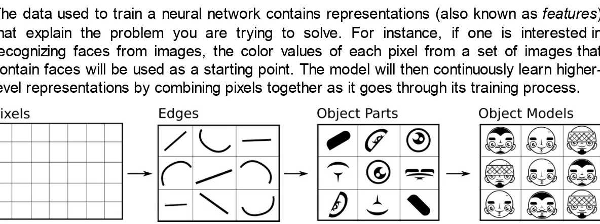
The data used to train a neural network contains representations (also known as features) that explain the problem you are trying to solve. For instance, if one is interested in recognizing faces from images, the color values of each pixel from a set of images that contain faces will be used as a starting point. The model will then continuously learn higher-level representations by combining pixels together as it goes through its training process.
Figure 1: Series of higher-level representations that begin on input data. Derivate image based on original image from: Yann LeCun, Yoshua Bengio & Geoffrey Hinton. "Deep Learning". Nature 521, 436–444 (28 May 2015) doi:10.1038/nature14539
In formal words, neural networks are computation graphs in which each step computes higher abstraction representations from input data.
Each one of these steps represents a progression into a different abstraction layer. Data progresses through these layers, building continuously higher-level representations. The process finishes with the highest representation possible: the one the model is trying to predict.
Function Approximation
When neural networks learn new representations of data, they do so by combining weights and biases with neurons from different layers. They adjust the weights of these connections e ve r y time a training cycle takes place using a mathematical technique called backpropagation. The weights and biases improve at each round, up to the point that an optimum is achieved. This means that a neural network can measure how wrong it is on every training cycle, adjust the weights and biases of each neuron, and try again. If it determines that a certain modification produces better results than the previous round, it will invest in that modification until an optimal solution is achieved.
In a nutshell, that procedure is the reason why neural networks can approximate functions. However, there are many reasons why a neural network may not be able to predict a function with perfection, chief among them being that:
Many functions contain stochastic properties (that is, random properties) There may be overfitting to peculiarities from the training data
There may be a lack of training data
with reasonable precision. These sorts of applications will be our focus throughout this data available for a given problem is either biased or only contains partial representations of the underlying functions that generate that problem, then deep learning techniques will only be able to reproduce the problem and not learn to solve it.
Remember that deep learning algorithms are learning different representations of data to approximate a given function. If data does not represent a function appropriately, it is likely that a function will be incorrectly represented by a neural network. Consider the following analogy: you are trying to predict the national prices of gasoline (that is, fuel) and create a deep learning model. You use your credit card statement with your daily expenses on gasoline as an input data for that model. The model may eventually learn the patterns of your gasoline consumption, but it will likely misrepresent price fluctuations of gasoline caused by other factors only represented weekly in your data such as government policies, market competition, international politics, and so on. The model will ultimately yield incorrect results when used in production.
To avoid this problem, make sure that the data used to train a model represents the problem the model is trying to address as accurately as possible.
Note
For an in-depth discussion of this topic, refer to François Chollet's upcoming book Deep Learning with Python. François is the creator of Keras, a Python library used in this book. The chapter, The limitations of deep learning, is particularly important for understanding this topic. The working version of that book is available at:
https://blog.keras.io/the-limitations-of-deep-learning.html.
Inherent Bias and Ethical Considerations
Researchers have suggested that the use of the deep learning model without considering the inherent bias in the training data can lead not only to poor performing solutions, but also to ethical complications.
convicted.
Note
Their model identified inmates with 89.5 percent accuracy. ( https://blog.keras.io/the-limitations-of-deep-learning.htmltations-of-deep-learning.html).
MIT Technology Review. Neural Network Learns to Identify Criminals by Their Faces. November 22, 2016. Available at: https://www.technologyreview.com/s/602955/neural-network-learns-to-identify-criminals-by-their-faces/.
The paper resulted in great furor within the scientific community and popular media. One key issue with the proposed solution is that it fails to properly recognize the bias inherent in the input data. Namely, the data used in this study came from two different sources: one for criminals and one for non-criminals. Some researchers suggest that their algorithm identifies patterns associated with the different data sources used in the study instead of identifying relevant patterns from people's faces. While there are technical considerations one can make about the reliability of the model, the key criticism is on ethical grounds: one ought to clearly recognize the inherent bias in input data used by deep learning algorithms and consider how its application will have an impact on people's lives.
Note
Timothy Revell. Concerns as face recognition tech used to 'identify' criminals. New
Scientist. December 1, 2016. Available at:
https://www.newscientist.com/article/2114900-concerns-as-face-recognition-tech-used-to-identify-criminals/.
For understanding more about the topic of ethics in learning algorithms (including deep learning), refer to the work done by the AI Now Institute (https://ainowinstitute.org/), an organization created for the understanding of the social implications of intelligent systems.
Common Components and Operations of Neural
Networks
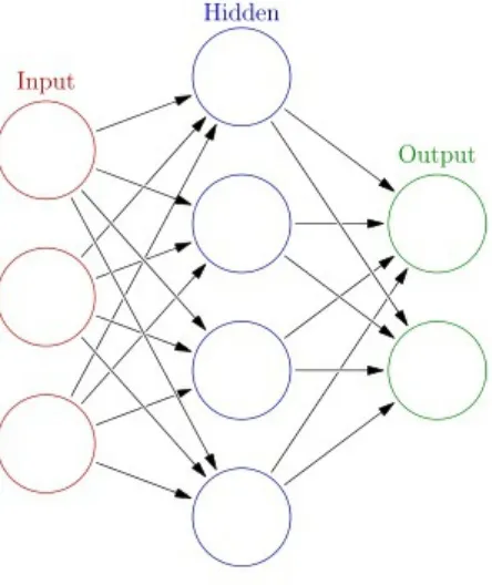
Neural networks have two key components: layers and nodes.
Input: Where the input data is received and first interpreted
Hidden: Where computations take place, modifying data as it goes through Output: Where an output is assembled and evaluated
Figure 2: Illustration of the most common layers in a neural network. By Glosser.ca - Own work, Derivative of File: Artificial neural network.svg, CC BY-SA 3.0, https://commons.wikimedia.org/w/index.php?curid=24913461
Hidden layers are the most important layers in neural networks. They are referred to as
hidden because the representations generated in them are not available in the data, but are learned from it. It is within these layers where the main computations take place in neural networks.
Nodes are where data is represented in the network. There are two values associated with nodes: biases and weights. Both of these values affect how data is represented by the nodes and passed on to other nodes. When a network learns, it effectively adjusts these values to satisfy an optimization function.
Most of the work in neural networks happens in the hidden layers. Unfortunately, there isn't a clear rule for determining how many layers or nodes a network should have. When implementing a neural network, one will probably spend time experimenting with different combinations of layers and nodes. It is advised to always start with a single layer and also with a number of nodes that reflect the number of features the input data has (that is, how many columns are available in a dataset). One will then continue to add layers and nodes until satisfactory performance is achieved—or whenever the network starts overfitting to the training data.
networks outperformed other algorithms simply by adjusting these parameters.
As an intuition, think about data entering a neural network system via the input layer, then moving through the network from node to node. The path that data takes will depend on how interconnected the nodes are, the weights and the biases of each node, the kind of operations that are performed in each layer, and the state of data at the end of such operations. Neural networks often require many "runs" (or epochs) in order to keep tuning the weights and biases of nodes, meaning that data flows over the different layers of the graph multiple times.
This section offered you an overview of neural networks and deep learning. Additionally, we discussed a starter's intuition to understand the following key concepts:
Neural networks can, in principle, approximate most functions, given that it has enough resources and data.
Layers and nodes are the most important structural components of neural networks. One typically spends a lot of time altering those components to find a working architecture.
Weights and biases are the key properties that a network "learns" during its training process.
Configuring a Deep Learning Environment
Before we finish this lesson, we want you to interact with a real neural network. We will start by covering the main software components used throughout this book and make sure that they are properly installed. We will then explore a pre-trained neural network and explore a few of the components and operations discussed earlier in the What are Neural Networks? section.
Software Components for Deep Learning
We'll use the following software components for deep learning:
Python 3
We will be using Python 3 in this book. Python is a general-purpose programming language which is very popular with the scientific community—hence its adoption in deep learning. Python 2 is not supported in this book but can be used to train neural networks instead of Python 3. Even if you chose to implement your solutions in Python 2, consider moving to Python 3 as its modern feature set is far more robust than that of its predecessor.
TensorFlow
TensorFlow is a library used for performing mathematical operations in the form of graphs. TensorFlow was originally developed by Google and today it is an open-source project with many contributors. It has been designed with neural networks in mind and is among the most popular choices when creating deep learning algorithms.
TensorFlow is also well-known for its production components. It comes with TensorFlow Serving (https://github.com/tensorflow/serving), a high-performance system for serving deep learning models. Also, trained TensorFlow models can be consumed in other high-performance programming languages such as Java, Go, and C. This means that one can deploy these models in anything from a micro-computer (that is, a RaspberryPi) to an Android device.
Keras
In order to interact efficiently with TensorFlow, we will be using Keras (https://keras.io/), a Python package with a high-level API for developing neural networks. While TensorFlow focuses on components that interact with each other in a computational graph, Keras focuses specifically on neural networks. Keras uses TensorFlow as its backend engine and makes developing such applications much easier.
It is available under the tf.keras namespace. If you have TensorFlow 1.4 or higher
installed, you already have Keras available in your system.
TensorBoard
TensorBoard is a data visualization suite for exploring TensorFlow models and is natively integrated with TensorFlow. TensorBoard works by consuming checkpoint and summary files created by TensorFlow as it trains a neural network. Those can be explored either in near real-time (with a 30 second delay) or after the network has finished training. TensorBoard makes the process of experimenting and exploring a neural network much easier—plus it's quite exciting to follow the training of your network!
Jupyter Notebooks, Pandas, and NumPy
When working to create deep learning models with Python, it is common to start working interactively, slowly developing a model that eventually turns into more structured software. Three Python packages are used frequently during that process: Jupyter Notebooks, Pandas, and NumPy:
Jupyter Notebooks create interactive Python sessions that use a web browser as its interface
Pandas is a package for data manipulation and analysis
NumPy is frequently used for shaping data and performing numerical computations
These packages are used occasionally throughout this book. They typically do not form part of a production system, but are often used when exploring data and starting to build a model. We focus on the other tools in much more detail.
Note
Python General-purpose programming language. Popularlanguage used in the development of deep learning
TensorFlow Open-source graph computation Python packagetypically used for developing deep learning systems. 1.4
Keras Python package that provides a high-level interface toTensorFlow. 2.0.8-tf(distributed with TensorFlow)
TensorBoard Browser-based software for visualizing neural networkstatistics. 0.4.0
Jupyter
Notebook Browser-based software for working interactively withPython sessions. 5.2.1
Pandas Python package for analyzing and manipulating data. 0.21.0
NumPy Python package for high-performance numericalcomputations. 1.13.3
Table 1: Software components necessary for creating a deep learning environment
Activity 1 – Verifying Software Components
Before we explore a trained neural network, let's verify that all the software components that we need are available. We have included a script that verifies these components work. Let's take a moment to run the script and deal with any eventual problems we may find.
We will now be testing if the software components required for this book are available in your working environment. First, we suggest the creation of a Python virtual environment using Python's native module venv. Virtual environments are used for managing project
dependencies. We advise each project you create to have its own virtual environments. Let's create one now.
Note
1. A Python virtual environment can be created by using the following command:
$ python3 -m venv venv $ source venv/bin/activate
2. The latter command will append the string (venv) to the beginning of your command
line. Use the following command to deactivate your virtual environment:
$ deactivate
Note
Make sure to always activate your Python virtual environment when working on a project.
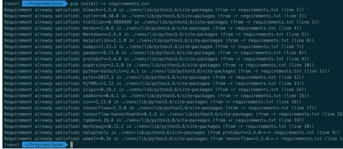
3. After activating your virtual environment, make sure that the right components are installed by executing pip over the file requirements.txt. This will attempt to install the
models used in this book in that virtual environment. It will do nothing if they are already available:
Figure 3: Image of a terminal running pip to install dependencies from requirements.txt
Install dependencies by running the following command:
$ pip install –r requirements.txt
this command should simply inform you.
These dependencies are essential for working with all code activities in this book.
As a final step on this activity, let's execute the script test_stack.py. That script
formally verifies that all the required packages for this book are installed and available in your system.
4. Students, run the script lesson_1/activity_1/test_stack.py to check if the
dependencies Python 3, TensorFlow, and Keras are available. Use the following command:
$ python3 lesson_1/activity_1/test_stack.py
The script returns helpful messages stating what is installed and what needs to be installed.
5. Run the following script command in your terminal:
$ tensorboard --help
You should see a help message that explains what each command does. If you do not see that message – or see an error message instead – please ask for assistance from your instructor:
Figure 4: Image of a terminal running python3 test_stack.py. The script returns messages informing that all dependencies are installed correctly.
Note
RuntimeWarning: compiletime version 3.5 of module
'tensorflow.python.framework.fast_tensor_util' does not match runtime version 3.6
return f(*args, **kwds)
That message appears if you are running Python 3.6 and the distributed TensorFlow wheel was compiled under a different version (in this case, 3.5). You can safely
For the reference solution, use the Code/Lesson-1/activity_1 folder.
Exploring a Trained Neural Network
In this section, we explore a trained neural network. We do that to understand how a neural network solves a real-world problem (predict handwritten digits) and also to get familiar with the TensorFlow API. When exploring that neural network, we will recognize many components introduced in previous sections such as nodes and layers, but we will also see many that we don't recognize (such as activation functions)—we will explore those in further sections. We will then walk through an exercise on how that neural network was trained and then train that same network on our own.
The network that we will be exploring has been trained to recognize numerical digits (integers) using images of handwritten digits. It uses the MNIST dataset (http://yann.lecun.com/exdb/mnist/), a classic dataset frequently used for exploring pattern recognition tasks.
MNIST Dataset
example, CIFAR). However, the MNIST dataset is still very useful for understanding how neural networks work because known models can achieve a high level of accuracy with great efficiency.
Note
Figure 5: Excerpt from the training set of the MNIST dataset. Each image is a separate 20x20 pixels image with a single handwritten digit. The original dataset is available at: http://yann.lecun.com/exdb/mnist/.
Training a Neural Network with TensorFlow
Now, let's train a neural network to recognize new digits using the MNIST dataset.
W = tf.Variable(
tf.truncated_normal([5, 5, size_in, size_out], stddev=0.1),
name="Weights")
B = tf.Variable(tf.constant(0.1, shape=[size_out]), name="Biases")
convolution = tf.nn.conv2d(input, W, strides=[1, 1, 1, 1], padding="SAME")
activation = tf.nn.relu(convolution + B) tf.nn.max_pool(
Use the mnist.py file for your reference at Code/Lesson-1/activity_2/. Follow along by
opening the script in your code editor.
We execute that snippet of code only once during the training of our network.
The variables W and B stand for weights and biases. These are the values used by the
nodes within the hidden layers to alter the network's interpretation of the data as it passes through the network. Do not worry about the other variables for now.
The fully connected layers are defined by the following snippet of Python code:
W = tf.Variable(
tf.truncated_normal([size_in, size_out], stddev=0.1), name="Weights")
B = tf.Variable(tf.constant(0.1, shape=[size_out]), name="Biases") activation = tf.matmul(input, W) + B
Note
Use the mnist.py file for your reference at Code/Lesson-1/activity_2/. Follow along by
opening the script in your code editor.
Here, we also have the two TensorFlow variables W and B. Notice how simple the
initialization of these variables is: W is initialized as a random value from a pruned Gaussian
distribution (pruned with size_in and size_out) with a standard deviation of 0.1, and B (the
each run. That snippet is executed twice, yielding two fully connected networks—one passing data to the other.
Those 11 lines of Python code represent our complete neural network. We will go into a lot more detail in Lesson 2, Model Architecture about each one of those components using Keras. For now, focus on understanding that the network is altering the values of W and B in
each layer on every run and how these snippets form different layers. These 11 lines of Python are the culmination of dozens of years of neural network research.
Let's now train that network to evaluate how it performs in the MNIST dataset.
Training a Neural Network
Follow the following steps to set up this exercise:
1. Open two terminal instances.
2. In both of them, navigate to the directory lesson_1/exercise_a.
3. In both of them, make sure that your Python 3 virtual environment is active and that the requirements outlined in requirements.txt are installed.
4. In one of them, start a TensorBoard server with the following command:
$ tensorboard --logdir=mnist_example/
5. In the other, run the train_mnist.py script from within that directory.
6. Open your browser in the TensorBoard URL provided when you start the server.
In the terminal that you ran the script train_mnist.py, you will see a progress bar with the
epochs of the model. When you open the browser page, you will see a couple of graphs. Click on the one that reads Accuracy, enlarge it and let the page refresh (or click on the refresh button). You will see the model gaining accuracy as epochs go by.
Use that moment to explain the power of neural networks in reaching a high level of accuracy very early in the training process.
We can see that in about 200 epochs (or steps), the network surpassed 90 percent accuracy. That is, the network is getting 90 percent of the digits in the test set correctly. The network continues to gain accuracy as it trains up to the 2,000th step, reaching a 97 percent accuracy at the end of that period.
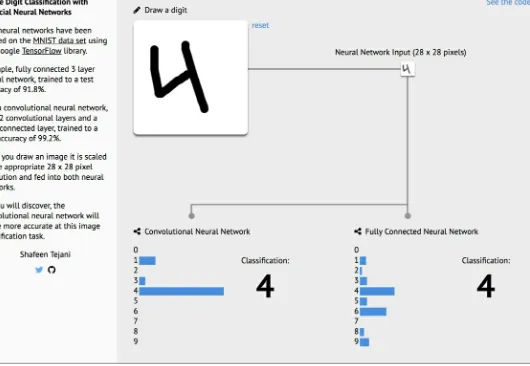
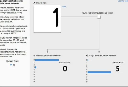
Now, let's also test how well those networks perform with unseen data. We will use an open-source web application created by Shafeen Tejani to explore if a trained network correctly predicts handwritten digits that we create.
Testing Network Performance with Unseen Data
Figure 6: Web application in which we can manually draw digits and test the accuracy of two trained netwo
Note
Source: https://github.com/ShafeenTejani/mnist-demo
Figure 7: Both networks have a difficult time estimating values drawn on the edges of the area
Note
In this example, we see the number 1 drawn to the right side of the drawing area. The probability of this number being a 1 is 0 in both networks.
The MNIST dataset does not contain numbers on the edges of images. Hence, neither network assigns relevant values to the pixels located in that region. Both networks are much better at classifying numbers correctly if we draw them closer to the center of the designated area. This shows that neural networks can only be as powerful as the data that is used to train them. If the data used for training is very different than what we are trying to predict, the network will most likely produce disappointing results.
Activity 2 – Exploring a Trained Neural Network
In this section, we will explore the neural network that we have trained during our exercis. We will also train a few other networks by altering hyperparameters from our original one.
trained network as binary files in the directory of this book. Let's open that trained network using TensorBoard and explore its components.
Using your terminal, navigate to the directory lesson_1/activity_2 and execute the
following command to start TensorBoard:
$ tensorboard --logdir=mnist_example/
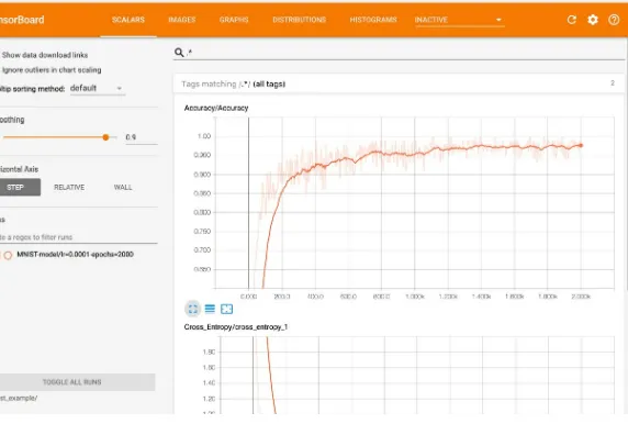
Now, open the URL provided by TensorBoard in your browser. You should be able to see the TensorBoard scalars page:
Figure 8: Image of a terminal after starting a TensorBoard instance
After you open the URL provided by the tensorboard command, you should be able to see
Figure 9: Image of the TensorBoard landing page
Let's now explore our trained neural network and see how it performed.
On the TensorBoard page, click on the Scalars page and enlarge the Accuracy graph. Now, move the Smoothing slider to 0.9.
The accuracy graph measures how accurate the network was able to guess the labels of a test set. At first, the network guesses those labels completely wrong. This happens because we have initialized the weights and biases of our network with random values, so its first attempts are a guess. The network will then change the weights and biases of its layers on a second run; the network will continue to invest in the nodes that give positive results by altering their weights and biases, and penalize those that don't by gradually reducing their impact on the network (eventually reaching 0). As you can see, this is a really
efficient technique that quickly yields great results.
Let's focus our attention on the Accuracy graph. See how the algorithm manages to reach great accuracy (> 95 percent) after around 1,000 epochs? What happens between 1,000 and 2,000 epochs? Would it get more accurate if we continued to train with more epochs?
a decreasing rate. The network may improve slightly if trained with more epochs, but it will not reach 100 percent accuracy with the current architecture.
The script is a modified version of an official Google script that was created to show how TensorFlow works. We have divided the script into functions that are easier to understand and added many comments to guide your learning. Try running that script by modifying the variables at the top of the script:
LEARNING_RATE = 0.0001 EPOCHS = 2000
Note
Use the mnist.py file for your reference at Code/Lesson-1/activity_2/.
Now, try running that script by modifying the values of those variables. For instance, try modifying the learning rate to 0.1 and the epochs to 100. Do you think the network can
achieve comparable results?
Note
There are many other parameters that you can modify in your neural network. For now, experiment with the epochs and the learning rate of your network. You will notice that those two on their own can greatly change the output of your network—but only by so much. Experiment to see if you can train this network faster with the current architecture just by altering those two parameters.
Summary
In this lesson, we explored a TensorFlow-trained neural network using TensorBoard and trained our own modified version of that network with different epochs and learning rates. This gave you hands-on experiences on how to train a highly performant neural network and also allowed you to explore some of its limitations.
Do you think we can achieve similar accuracy with real Bitcoin data? We will attempt to predict future Bitcoin prices using a common neural network algorithm during Lesson 2,
Chapter 2. Model Architecture
Building on fundamental concepts from Lesson 1, Introduction to Neural Networks and Deep Learning, we now move into a practical problem: can we predict Bitcoin prices using a deep learning model? In this lesson, we will learn how to build a deep learning model that attempts to do that.
We will conclude this lesson by putting all of these components together and building a bare-bones yet complete first version of a deep learning application.
Lesson Objectives
In this lesson, you will:
Prepare data for a deep learning model Choose the right model architecture
Choosing the Right Model Architecture
Deep learning is a field undergoing intense research activity. Among other things, researchers are devoted to inventing new neural network architectures that can either tackle new problems or increase the performance of previously implemented architectures.
In this section, we study both old and new architectures. Older architectures have been used to solve a large array of problems and are generally considered the right choice when starting a new project. Newer architectures have shown great successes in specific problems, but are harder to generalize. The latter are interesting as references of what to explore next, but are hardly a good choice when starting a project.
Common Architectures
Considering the many architecture possibilities, there are two popular architectures that have often been used as starting points for a number of applications: convolutional neural networks (CNNs) and recurrent neural networks (RNNs). These are foundational networks and should be considered starting points for most projects. We also include descriptions of another three networks, due to their relevance in the field: Long-short term memory (LSTM) networks, an RNN variant; generative adversarial networks (GANs); and deep reinforcement learning. These latter architectures have shown great successes in solving contemporary problems, but are somewhat more difficult to use.
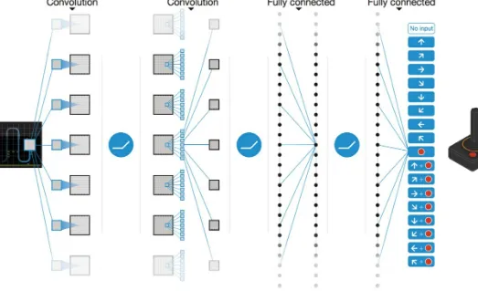
Convolutional Neural Networks
Convolutional neural networks have gained notoriety for working with problems that have a grid-like structure. They were originally created to classify images, but have been used in a number of other areas, ranging from speech recognition to self-driving vehicles.
CNN's essential insight is to use closely related data as an element of the training process, instead of only individual data inputs. This idea is particularly effective in the context of images, where a pixel located to the right of another pixel is related to that pixel as well, given that they form part of a larger composition. In this case, that composition is what the network is training to predict. Hence, combining a few pixels together is better than using an individual pixel on its own.
Figure 1: Illustration of the convolution process Image source: Volodymyr Mnih, et al.
Note
For more information refer, Human-level control through deep reinforcement learning. February 2015, Nature. Available at: https://storage.googleapis.com/deepmind-media/dqn/DQNNaturePaper.pdf.
Recurrent Neural Networks
Convolutional neural networks work with a set of inputs that keep altering the weights and biases of the networks' respective layers and nodes. A known limitation of this approach is that its architecture ignores the sequence of these inputs when determining how to change the networks' weights and biases.
Recurrent neural networks were created precisely to address that problem. RNNs are designed to work with sequential data. This means that at every epoch, layers can be influenced by the output of previous layers. The memory of previous observations in a given sequence plays a role in the evaluation of posterior observations.
another.
Note
For more information refer, Transformer: A Novel Neural Network Architecture for Language Understanding, by Jakob Uszkoreit, Google Research Blog, August 2017. Available at: https://research.googleblog.com/2017/08/transformer-novel-neural-network.html.
Figure 2: Illustration from distill.pub (https://distill.pub/2016/augmented-rnns/)
Figure 2 shows that words in English are related to words in French, based on where they appear in a sentence. RNNs are very popular in language translation problems.
Long-short term memory networks are RNN variants created to address the vanishing gradient problem. The vanishing gradient problem is caused by memory components that are too distant from the current step and would receive lower weights due to their distance. LSTMs are a variant of RNNs that contain a memory component—called forget gate. That component can be used to evaluate how both recent and old elements affect the weights and biases, depending on where the observation is placed in a sequence.
Note
For more details refer, The LSTM architecture was first introduced by Sepp Hochreiter and Jürgen Schmidhuber in 1997. Current implementations have had several modifications. For a detailed mathematical explanation of how each component of an LSTM works, we suggest the article Understanding LSTM Networks by Christopher Olah, August 2015, available at http://colah.github.io/posts/2015-08-Understanding-LSTMs/.
Generative Adversarial Networks
his colleagues at the University of Montreal. GANs suggest that, instead of having one neural network that optimizes weights and biases with the objective to minimize its errors, there should be two neural networks that compete against each other for that purpose.
Note
For more details refer, Generative Adversarial Networks by Ian Goodfellow, et al, arXiv. June 10, 2014. Available at: https://arxiv.org/abs/1406.2661.
GANs have a network that generates new data (that is, "fake" data) and a network that evaluates the likelihood of the data generated by the first network to be real or "fake". They compete because both learn: one learns how to better generate "fake" data, and the other learns how to distinguish if the data it is presented with is real or not. They iterate on every epoch until they both converge. That is the point when the network that evaluates generated data cannot distinguish between "fake" and real data any longer.
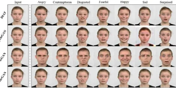
GANs have been successfully used in fields where data has a clear topological structure. Its original implementation used a GAN to create synthetic images of objects, people's faces, and animals that were similar to real images of those things. This domain of image creation is where GANs are used the most frequently, but applications in other domains occasionally appear in research papers.
Figure 3: Image that shows the result of different GAN algorithms in changing people's faces based on a given emotion. Source: StarGAN Project. Available at https://github.com/yunjey/StarGAN.
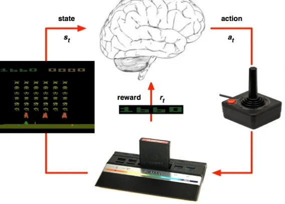
The original DRL architecture was championed by DeepMind, a Google-owned artificial intelligence research organization based in the UK. The key idea of DRL networks is that they are unsupervised in nature and that they learn from trial-and-error, only optimizing for a reward function. That is, different than other networks (which use supervised approaches to optimize for how wrong the predictions are, compared to what is known to be right), DRL networks do not know of a correct way of approaching a problem. They are simply given the rules of a system and are then rewarded every time they perform a function correctly. This process, which takes a very large number of iterations, eventually trains networks to excel in a number of tasks.
Note
For more information refer, Human-level control through deep reinforcement learning, by Volodymyr Mnih et al., February 2015, Nature. Available at:
https://storage.googleapis.com/deepmind-media/dqn/DQNNaturePaper.pdf.
Figure 4: Image that represents how the DQN algorithm works
Note
For more information refer, DQN was created by DeepMind to beat Atari games. The algorithm uses a deep reinforcement learning solution to continuously increase its reward. Image source: https://keon.io/deep-q-learning/.
Architecture Data Structure SuccessfulApplications
Convolutional neural networks
Recurrent neural network (RNN) and long-short term memory (LSTM) networks
Sequential data (that is,
time-series data) Speech recognition,text generation, and translation
Generative adversarial networks
(GANs) Grid-like topologicalstructure (that is, images) Image generation
Deep reinforcement learning (DRL) System with clear rules anda clearly defined reward function
Playing video games and self-driving vehicles
Table 1: Different neural network architectures have shown success in different fields. The networks' architecture is typically related to the structure of the problem at hand.
Data Normalization
Before building a deep learning model, one more step is necessary: data normalization.
Data normalization is a common practice in machine learning systems. Particularly regarding neural networks, researchers have proposed that normalization is an essential technique for training RNNs (and LSTMs), mainly because it decreases the network's training time and increases the network's overall performance.
Note
For more information refer, Batch Normalization: Accelerating Deep Network Training by Reducing Internal Covariate Shift by Sergey Ioffe et. al., arXiv, March 2015. Available at: https://arxiv.org/abs/1502.03167.
Deciding on a normalization technique varies, depending on the data and the problem at hand. The following techniques are commonly used.
Z-score
Here, is the observation, the mean, and the standard deviation of the series.
Note
For more information refer, Standard score article (Z-score). Wikipedia. Available at:
https://en.wikipedia.org/wiki/Standard_score.
Point-Relative Normalization
This normalization computes the difference of a given observation in relation to the first observation of the series. This kind of normalization is useful to identify trends in relation to a starting point. The point-relative normalization is defined by:
Here, is the observation and is the first observation of the series.
Note
As suggested by Siraj Raval in his video, How to Predict Stock Prices Easily - Intro to Deep Learning #7, available on YouTube at: https://www.youtube.com/watch? v=ftMq5ps503w.
This normalization computes the distance between a given observation and the maximum and minimum values of the series. This normalization is useful when working with series in which the maximum and minimum values are not outliers and are important for future predictions. This normalization technique can be applied with:
Here, is the observation, O represents a vector with all O values, and the functions min (O) and max (O) represent the minimum and maximum values of the series, respectively.
During Activity 3, Exploring the Bitcoin Dataset and Preparing Data for Model, we will prepare available Bitcoin data to be used in our LSTM mode. That includes selecting variables of interest, selecting a relevant period, and applying the preceding point-relative normalization technique.
Structuring Your Problem
Compared to researchers, practitioners spend much less time determining which architecture to choose when starting a new deep learning project. Acquiring data that represents a given problem correctly is the most important factor to consider when developing these systems, followed by the understanding of the dataset's inherent biases and limitations.
When starting to develop a deep learning system, consider the following questions for reflection:
Do I have the right data? This is the hardest challenge when training a deep learning model. First, define your problem with mathematical rules. Use precise definitions and organize the problem in either categories (classification problems) or a continuous scale (regression problems). Now, how can you collect data about those metrics?
Do I have enough data? Typically, deep learning algorithms have shown to perform much better in large datasets than in smaller ones. Knowing how much data is necessary to train a high-performance algorithm depends on the kind of problem you are trying to address, but aim to collect as much data as you can.
Figure 5: Decision-tree of key reflection questions to be made at the beginning of a deep learning project
In certain circumstances, data may simply not be available. Depending on the case, it may be possible to use a series of techniques to effectively create more data from your input data. This process is known as data augmentation and has successful application when working with image recognition problems.
Note
A good reference is the article Classifying plankton with deep neural networks available a t http://benanne.github.io/2015/03/17/plankton.html. The authors show a series of techniques for augmenting a small set of image data in order to increase the number of training samples the model has.
Activity 3 – Exploring the Bitcoin Dataset and
Preparing Data for Model
We will be using a public dataset originally retrieved from CoinMarketCap, a popular website that tracks different cryptocurrency statistics. The dataset has been provided alongside this lesson and will be used throughout the rest of this book.
We will be exploring the dataset using Jupyter Notebooks. Jupyter Notebooks provide Python sessions via a web-browser that allows you to work with data interactively. They are a popular tool for exploring datasets. They will be used in activities throughout this book.
Using your terminal, navigate to the directory lesson_2/activity_3 and execute the
following command to start a Jupyter Notebook instance:
$ jupyter notebook
Now, open the URL provided by the application in your browser. You should be able to see a Jupyter Notebook page with a number of directories from your file system.
Figure 6: Terminal image after starting a Jupyter Notebook instance. Navigate to the URL show in a browser, and you should be able to see the Jupyter Notebook landing page.
Now, navigate to the directories and click on the file
Activity_3_Exploring_Bitcoin_Dataset.ipynb. This is a Jupyter Notebook file that will be
opened in a new browser tab. The application will automatically start a new Python interactive session for you.
Figure 8: Image of the Notebook Activity_3_Exploring_Bitcoin_Dataset.ipynb. You can now interact with that Notebook and make modifications.
After opening our Jupyter Notebook, let's now explore the Bitcoin data made available with this lesson.
The dataset data/bitcoin_historical_prices.csv contains measurements of Bitcoin
prices since early 2013. The most recent observation is on November 2017—the dataset comes from CoinMarketCap, an online service that is updated daily. It contains eight variables, two of which (date and week) describe a time period of the data—these can be
used as indices—and six others (open, high, low, close, volume, and market_capitalization) that can be used to understand how the price and value of Bitcoin
has changed over time:
Variable Description
date Date of the observation.
open Open value for a single Bitcoin coin.
high Highest value achieved during a given day period.
low Lowest value achieved during a given day period.
close Value at the close of the transaction day.
volume The total volume of Bitcoin that was exchanged during that day.
market_capitalization Market capitalization, which is explained by Circulating Supply. Market Cap = Price *
Table 2: Available variables (that is, columns) in the Bitcoin historical prices dataset
Using the open Jupyter Notebook instance, let's now explore the time-series of two of those variables: close and volume. We will start with those time-series to explore price-fluctuation
patterns.
Navigate to the open instance of the Jupyter Notebook
Activity_3_Exploring_Bitcoin_Dataset.ipynb. Now, execute all cells under the header
Introduction. This will import the required libraries and import the dataset into memory.
After the dataset has been imported into memory, move to the Exploration section. You will find a snippet of code that generates a time-series plot for the close variable. Can you
Figure 9: Time-series plot of the closing price for Bitcoin from the close variable. Reproduce this plot, but using the volume variable in a new cell below this one.
You will have most certainly noticed that both variables surge in 2017. This reflects the current phenomenon that both the prices and value of Bitcoin have been continuously growing since the beginning of that year.
recent prices have skyrocketed since the beginning of 2017.
Figure 11: The volume of transactions of Bitcoin coins (in USD) shows that starting in 2017, a trend starts in which a significantly larger amount of Bitcoin is being transacted in the market. The total daily volume varies much more than daily
closing prices.
Also, we notice that for many years, Bitcoin prices did not fluctuate as much as in recent years. While those periods can be used by a neural network to understand certain patterns, we will be excluding older observations, given that we are interested in predicting future prices for not-too-distant periods. Let's filter the data for 2016 and 2017 only.
Navigate to the Preparing Dataset for Model section. We will use the pandas API for
filtering the data for the years 2016 and 2017. Pandas provides an intuitive API for performing this operation:
bitcoin_recent = bitcoin[bitcoin['date'] >= '2016-01-01']
The variable bitcoin_recent now has a copy of our original bitcoin dataset, but filtered to
the observations that are newer or equal to January 1, 2016.
As our final step, we now normalize our data using the point-relative normalization technique described in the Data Normalization section. We will only normalize two variables (close
and volume), because those are the variables that we are working to predict.
In the same directory containing this lesson, we have placed a script called
normalizations.py. That script contains the three normalization techniques described in
this lesson. We import that script into our Jupyter Notebook and apply the functions to our series.
Navigate to the Preparing Dataset for Model section. Now, use the iso_week variable to
group all the day observations from a given week using the pandas method groupby(). We
can now apply the normalization function
normalizations.point_relative_normalization() directly to the series within that week.
using:
bitcoin_recent['close_point_relative_normalization'] = bitcoin_recent.groupby('iso_week')['close'].apply(
lambda x: normalizations.point_relative_normalization(x))
The variable close_point_relative_normalization now contains the normalized data for
the variable close. Do the same with the variable volume:
Figure 12: Image of Jupyter Notebook focusing on section where the normalization function is applied
The normalized close variable contains an interesting variance pattern every week. We will
Figure 13: Plot that displays the series from the normalized variable close_point_relative_normalization
In order to evaluate how well our model performs, we need to test its accuracy versus some other data. We do that by creating two datasets: a training set and a test set. In this activity, we will use 80 percent of the dataset to train our LSTM model and 20 percent to evaluate its performance.
Given that the data is continuous and in the form of a time series, we use the last 20 percent of available weeks as a test set and the first 80 percent as a training set: