Modelling, interpolation and stochastic simulation in
space and time of global solar radiation
Luca Bechini
a,∗, Giorgio Ducco
b,1, Marcello Donatelli
c,2, Alfred Stein
d,3aIstituto di Agronomia, Università degli Studi, Via Celoria 2, 20133 Milano, Italy bARPA Emilia-Romagna, Viale Silvani 6, 40122 Bologna, Italy
cIstituto Sperimentale per le Colture Industriali, Via di Corticella 133, 40128 Bologna, Italy dLaboratory of Soil Science and Geology, Department of Environmental Sciences, Wageningen University,
P.O. Box 37, 6700 AA Wageningen, The Netherlands
Received 15 July 1999; received in revised form 3 November 1999; accepted 2 December 1999
Abstract
Global solar radiation data used as daily inputs for most cropping systems and water budget models are frequently available from only a few weather stations and over short periods of time. To overcome this limitation, the Campbell–Donatelli model relates daily maximum and minimum air temperatures to solar radiation. In this study, calibrated values of model site specific parameters and efficiencies of radiation estimates are reported for 29 stations in northern Italy. Their average root mean squared error equals 2.9 MJ m−2per day. Model inputs and model output show a clear spatial and temporal structure. For
large scale model application, atmospheric transmissivity is calculated with ‘calculate first, interpolate later’ (CI) procedures and ‘interpolate the inputs, calculate later’ (IC) procedures. The mean squared error for CI equals 0.0359, whereas that for IC equals 0.0636. Comparison of ‘calculate first, simulate later’ (CS) procedures with ‘simulate the inputs, calculate later’ (SC) procedures shows a higher spatial sensitivity of SC procedures. The study shows how the model can be best applied to estimate global solar radiation, both at visited and unvisited locations, over a large and productive agricultural area in Italy, and hence, to better use water budget/crop productivity models. In addition, CS procedures show the associated error. © 2000 Elsevier Science B.V. All rights reserved.
Keywords: Model application; Regional-scale modelling; Northern Italy; Geostatistics; Simulated annealing; Space–time statistics;
Spatial-temporal simulations; Solar radiation; Parameter interpolation
∗Corresponding author. Tel.:+39-02-70600164;
fax:+39-02-70633243.
E-mail addresses: [email protected] (L. Bechini),
[email protected] (G. Ducco), [email protected] (M. Donatelli), [email protected] (A. Stein)
1Tel.:+39-0171-48678; fax:+39-051-284664. 2Tel.:+39-051-6316843; fax:+39-051-374857. 3Tel.:+31-0317-482420; fax:+31-0317-482419.
1. Introduction
The use of cropping systems and water budget mod-els requires global solar radiation as a daily input for estimation of potential evapotranspiration and crop biomass accumulation. Solar radiation data are diffi-cult and expensive to measure. Moreover, their repre-sentativeness for areas of land and periods of time is generally unknown. In Italy, reliable radiation data are available from a few meteorological stations only and
over short periods of time (<10 years). This can be a severe limitation for agricultural models application.
To overcome this limitation, research has been car-ried out in the past to model the physical relation be-tween maximum and minimum temperatures. These models use the daily air temperature range to estimate atmospheric transmissivity: on the one hand, cloud cover decreases daily maximum temperature because of the smaller input of short wave radiation; on the other hand, cloud cover increases the minimum air temperature during night time because of the greater emissivity of clouds compared to a clear sky. Exam-ples of this approach are the works of Brinsfield et al. (1984), Bristow and Campbell (1984), Hargreaves et al. (1985), Donatelli and Marletto (1994), Donatelli and Campbell (1998). Other methods also use rainfall measurements (Hodges et al., 1985; Reddy, 1987; McCaskill, 1990; Bindi and Miglietta, 1991; Hook and McClendon, 1992; Nikolov and Zeller, 1992; Elizondo et al., 1994). Hunt et al. (1998) compared several of the above methods.
The model proposed by Donatelli and Campbell (1998) has a strong physical basis, requires only clear sky transmissivity and maximum and minimum tem-peratures, is simply implemented in any spreadsheet or programming language and has proven to perform better than other models. For these reasons, it was cho-sen for application in this study.
Solar radiation models can be applied at individual stations. For a large scale application, however, mod-elled solar radiation must be interpolated. The question emerges whether it is better to first apply the model to point observations of input values and then interpolate the outputs (calculate first, interpolate later, CI) or to interpolate input values towards a grid and apply the model with these inputs (interpolate first, calculate later, IC, Stein et al., 1991). When models are not lin-ear, IC procedures should be preferred, even if accu-rate interpolation of inputs is then needed. Interpolated data, though, are smoothed (Journel and Huijbregts, 1978), and geostatistical simulations better represent actual spatial variation. These procedures can be read-ily applied to analyse quantitative error propagation. In addition, spatial simulations of modelled solar radi-ation show the effects of spatial variradi-ation on the model output. Again, two approaches can be distinguished: simulate input data first, followed by model calcula-tions (SC), or calculate radiation data first, followed
by their simulation (CS). The SC procedure yields a spatial uncertainty analysis by means of a Monte Carlo simulation, the CS procedure represents the actually occurring spatial-temporal variation of calculated radiation.
The objective of this study was to provide reliable methods for estimating radiation in northern Italy at a regional scale by:
• calibrating the model proposed by Donatelli and Campbell (1998) at 29 locations in northern Italy; • identifying the spatial structure of model parameters
and of the weather variables;
• comparing CI and IC procedures for model appli-cation in northern Italy;
• explore the use of CS and SC procedures for spa-tial error propagation and representation of spaspa-tial variation, respectively.
The study uses an extensive database collected in northern Italy.
2. Materials and methods
2.1. The model
The model proposed by Donatelli and Campbell (1998) estimates the actual atmospheric transmissivity (tti) for the ith day of the year as a function of clear sky transmissivity (τ) and daily maximum (Tmaxi) and minimum (Tmini) temperatures
tem-perature factor). High Tnc values decrease the effect of Tmin, and vice versa, by means of the exponential function g(Tmin). The parameter Tnc is active only if
Tmin reaches a high value, whereas for low Tmin the value of g(Tmin)≈1. Daily actual radiation is then ob-tained by multiplying daily potential radiation for a given day and latitude (Bristow and Campbell, 1984) by the atmospheric transmissivity tti.
The parameters b and Tncwere calibrated by using all the data available at each location (Table 1), by cal-culating the lowest root mean squared error (RMSE) between observed and measured data (Loague and Green, 1991).
2.2. Data collection
Daily maximum and minimum temperatures and global solar radiation have been obtained for 29 weather stations in northern Italy (Table 1, Fig. 1).
Several years of data were available for each station. A quality data check was performed on the data: • radiation values below 0.01 MJ m−2 per day or
above the potential for the given day and latitude (assuming τ=0.8) were considered wrong and therefore excluded from analysis;
• τ was calculated for each location, by averaging the five highest atmospheric transmissivities between day of year 120 and day of year 240 (for a given day, τ=MR/PR, with MR the measured radiation and PR the potential radiation). Stations with τ <0.71 have been considered affected by a systematic er-ror in measurements (Iqbal, 1983); their measured radiation data were then multiplied by a coefficient to obtainτ=0.71.
2.3. Comparison between measured and estimated solar radiations
After calibration of b and Tnc, global solar radia-tion was estimated with the model for all years and stations. Agreement between measured and predicted values was described by: the slope and the coefficient of determination (R2) of the regression line between predicted and observed values and by the RMSE, the modelling efficiency (ME) and the coefficient of resid-ual mass (CRM), the latter two as described by Loague and Green (1991).
2.4. Geostatistical procedures
The variables analysed in this study are related to their position in space, and are hence called geo-variables, denoted by Z(x, t), where Z is the prop-erty, such as Tmin, Tmax and tti, x the location in the two-dimensional study area, characterised by co-ordinates measured with respect to an arbitrary ori-gin, and t is the day of the year. Observations on Z(x,
t) are denoted by z(xi, tj), i=1,. . ., 29; j=1,. . ., 365. Regionalised variables and their unknown spatial and temporal variation can be modelled with random func-tions. Random functions are characterised, among other measures, by the first and second moment. From the first moment, one knows whether Z(x, t) shows a trend. From the second moment, one knows whether its variance exists, is independent upon loca-tion and time, and shows a dependence as a funcloca-tion of the spatial distance or the time interval. Usually a stronger similarity exists between nearby locations and for small intervals of time than between far-off locations and for long interval of time. A convenient way of modelling this dependence for variables with-out a trend is the variogram, defined as a function of the distance hs and the interval of time ht:
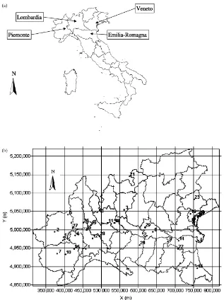
Fig. 1. (a) Position of the study area in Italy: the weather stations are located in following regions of northern Italy: Piemonte, Lombardia, Emilia-Romagna, Veneto; (b) Position of weather stations where the data used in this study were collected. Coordinates are expressed with Gauss-Boaga coordinate system. The boundaries of several provinces of northern Italy are represented.
we use simulated annealing (Kirkpatrick et al., 1983; Deutsch and Journel, 1998). The data used (29 points in space) did not allow to study anisotropy.
2.4.1. Calculate first, interpolate later
Input data, Tmax and Tmin, observed at individual points, allow to calculate atmospheric transmissivities.
com-binations of 1994 (25% of data available for 1994). A linear variogram model was fitted to the calculated spatio-temporal variogram of the modelled transmis-sivity, where distance was expressed as the square root of a function of hs and ht
γ (hs, ht)=C0+C(h2s +ϕh2t)1/2 (4) To estimate model parameters C0, C1 and ϕ, a weighted constrained non-linear regression with a se-quential quadratic programming algorithm was used. All parameters were bounded to be >0. The model was validated by interpolating (with OK) the calculated atmospheric transmissivity towards the independent test set of 5268 place–day combinations not used for variogram estimation.
The mean squared error (MSE) was calculated at the test points as
MSE=
Pn
i=1(ttp−tto)2
n (5)
where ttp is the daily atmospheric transmissivity predicted with the interpolation, tto is the observed daily atmospheric transmissivity and n=5628. Also, the mean variance of the prediction error (MVP) or kriging error variance was calculated as
MVP=
Pn
i=1var(ttp−tts)
n (6)
where tts is the value for the stochastic geovariable.
2.4.2. Interpolate first, calculate later
Input data (b, Tnc,τ,Tmaxi,Tmini andTmini+1) are interpolated towards grid nodes covering the study area, followed by model calculations at each of these nodes. This leads to the so-called IC procedures. For each input variable, the most convenient interpolation procedure is selected.
For the IC procedure, variograms were computed for the b, Tncandτ parameters in the spatial domain and daily temperatures in the spatio-temporal domain, by using the same 1606 randomly selected place–day combinations used for the CI procedure. The param-eters b, Tnc and τ were interpolated in space, while daily temperatures were interpolated in space and time towards the 5628 test points. The model was applied to the interpolated inputs to calculate atmospheric trans-missivity, then MSE was calculated. A comparison of
MSE obtained with CI and IC procedures provide sug-gestions for model application at regional scale.
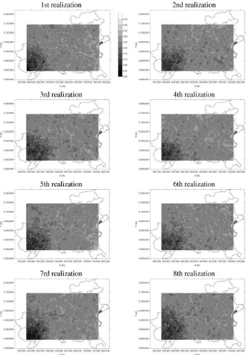
2.4.3. Calculate first, simulate later
Model outputs are conditionally simulated for the study area, the so-called CS procedure. Simulations are equivalent to simulated realisations of the random space function. They are useful, like the kriging vari-ance, to get an impression of the region of the high-est uncertainty, but do not require any assumption on Gaussianity.
2.4.4. Simulate first, calculate later
Conditional simulations of the input variables were used to analyze model uncertainty for spatial variation of the input variables. Input variables are simulated towards the nodes of a fine-meshed grid, followed by model calculations at each of these grid nodes. Upon comparison of many of these model calculations, an impression can be obtained as concerns the spatial uncertainty. This leads to the so-called SC procedures. For the four procedures, atmospheric transmissiv-ity instead of radiation has been chosen as the test variable because it meets the intrinsic hypothesis (the expectation of the geovariable is constant).
3. Results
3.1. Model calibration
Table 1 shows calibration of the b and Tnc param-eters. Summary statistics forτ, b, Tncare reported in Table 2.τis rather stable across the studied area, while
b and Tncshow higher variability. The coefficient of
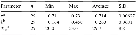
Table 2
Calibration of the Campbell–Donatelli model: summary statistics for calibrated model parameters (τ, b and Tnc)
Parameter n Min Max Average S.D.
τa 29 0.71 0.73 0.714 0.00627
bb 29 0.164 0.450 0.263 0.0681
Tncc 29 20.0 53.0 29.7 8.8 aτ: Cleary sky atmospheric transmissivity.
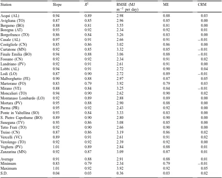
Table 3
Model performance at 29 weather stations: comparison between observed and predicted daily global solar radiation valuesa
Station Slope R2 RMSE (MJ
m−2 per day)
ME CRM
Acqui (AL) 0.94 0.89 2.98 0.88 0.03
Avigliana (TO) 0.87 0.85 2.96 0.85 0.00
Bergamo (BG) 0.88 0.81 3.55 0.81 0.00
Boregna (AT) 0.93 0.92 2.34 0.92 0.01
Borgofranco (TO) 0.86 0.84 3.26 0.83 0.00
Casale (AL) 0.97 0.91 2.66 0.91 −0.01
Costigliole (CN) 0.85 0.86 3.02 0.86 0.00
Curtatone (MN) 0.92 0.85 3.32 0.85 −0.01
Finale Emilia (BO) 0.94 0.88 3.06 0.88 −0.01
Fossano (CN) 0.92 0.92 2.34 0.91 0.02
Landriano (PV) 0.92 0.91 2.61 0.91 0.00
Lobbi (AL) 0.94 0.91 2.72 0.90 0.04
Lodi (LO) 0.87 0.90 2.72 0.89 −0.01
Malborghetto (FE) 0.90 0.88 2.97 0.87 0.05
Martorano (FO) 0.83 0.79 3.92 0.79 0.03
Mirano (VE) 0.88 0.84 3.25 0.84 −0.01
Moncalieri (TO) 0.94 0.90 2.62 0.90 0.02
Montanaso Lombardo (LO) 0.92 0.89 2.88 0.89 0.00
Mortara (PV) 0.95 0.88 2.90 0.88 0.00
Parma (PR) 0.95 0.92 2.43 0.92 0.00
Ponte in Valtellina (SO) 0.93 0.84 3.33 0.83 0.00
S. Pietro Capofiume (BO) 0.89 0.90 2.80 0.90 0.00
Susegana (TV) 0.93 0.86 3.08 0.85 0.00
Tetto Frati (TO) 0.92 0.90 2.66 0.90 0.00
Treiso (CN) 0.87 0.86 3.19 0.86 0.02
Vercelli (VC) 0.89 0.91 2.61 0.91 0.02
Verolengo (TO) 0.92 0.92 2.39 0.92 0.00
Voghera (PV) 1.01 0.89 2.84 0.88 0.01
Zanzarina (MN) 0.92 0.87 3.09 0.87 0.01
Average 0.91 0.88 2.91 0.88 0.01
Minimum 0.83 0.79 2.34 0.79 −0.01
Maximum 1.01 0.92 3.92 0.92 0.05
S.D. 0.04 0.03 0.36 0.03 0.02
aR2: the slope and the coefficient of determination of the regression line between predicted and observed values; RMSE: root mean squared error; ME: modelling efficiency; CRM: coefficient of residual mass (Loague and Green, 1991).
variation is very similar for b and Tnc. Higher values for b frequently occur at stations of higher altitudes. Low values for Tnc (between 20 and 23◦C) are typi-cal for low-level plain locations, where the effect of reduced night air cooling is more evident.
Table 3 shows the statistical indices obtained by comparing modelled and measured global solar radiation. Model performance is satisfactory for most locations; the average value for the slope of the regres-sion line between observed and measured radiation is 0.91, R2 is 0.88 and the RMSE ranges from 2.3 to 3.9 MJ m−2per day.
Other RMSE values found by other authors using similar methods equal 3.4–4.1 (Hunt et al., 1998), 3 (Bristow and Campbell, 1984), 2.9–3.6 (Elizondo et al., 1994), 3.4–5.2 (McCaskill, 1990), 3.5–5.6 (Supit, 1994) and 3.2–5.9 (Bindi et al., 1996).
3.2. Geostatistics
3.2.1. CI procedure
Table 4
Large scale model application: variogram model parameters for calculated atmospheric transmissivity and maximum and minimum temperatures (Tmax and Tmin)a
Variable Procedure C0 C1 ϕ R2 MSE MVP aThe linear variogram model is described in Eq. (4); asymptotic 95% confidence intervals are indicated in parenthesis; tt
i: calculated
atmospheric transmissivity; Tmax: maximum temperature; Tmin: minimum temperature; C0: nugget effect; C1: slope;ϕ: coefficient accounting for distance in time; MSE: mean squared error calculated by comparing calculated and observed independent data; MVP: kriging error variance; CI: ‘calculate first, interpolate later’ procedure; IC: ‘interpolate the inputs, calculate later’ procedure.
values obtained for model parameters are given in Table 4.
Atmospheric transmissivity shows a weak spatial dependence and a high nugget, showing that spatial variability is nearly the same over the whole area. This is probably related to variability at scales smaller than the average sampling interval and can limit the results of the methodology applied. Moreover, the variable shows a clear time dependence with a range at about 75–80 days. Validation against the independent data set yielded the results shown in Table 5.
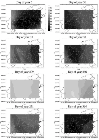
As an application example, the calculated atmo-spheric transmissivity was interpolated for 10 ran-domly selected days of year 1994 (Fig. 2) on a grid of 40×26 nodes.
Spatial variation is clearly present at individual days, with very high transmissivity at the (summer) Days 209 and 246, a rather temporal variation is visi-ble. Even on three consecutive days (36, 37 and 38) an interesting change in the pattern is visible, with (relatively) high transmissivity in the eastern part of the area on Day 36, and on the western part of the area on Days 37 and 38.
Table 5
Large scale model application: comparison of CI (calculate first, interpolate later) and IC (interpolate the inputs, calculate later) procedures
MSE MVP
CI 0.0359 0.08551
IC 0.06361 –
3.2.2. IC procedure
No spatial trend was found for the empirical para-meters b and Tnc, and for τ. A pure nugget effect was identified as the spatial structure forτ (nugget= 4.917×10⁻⁵), while for the empirical parameters the variogram models are described in Table 6.
For daily temperatures, variograms are calculated using four lags of 60 km in space and 10 lags of 15 days in time. The same spatio-temporal linear vario-gram model used for transmissivity was fitted, yield-ing the parameters shown in Table 4. All coefficients are not significantly different from zero. Variogram models for b and Tnc were cross-validated, yielding an MSE value of 0.005 for b and 58.911 for Tnc (Table 6). The space–time variogram models obtained for Tmaxand Tminwere validated against the indepen-dent data set (Table 4).
Finally, to carry out model calculations on the 5628 test points, interpolated daily temperatures in space and time and interpolated b and Tnc values in space were used. Estimates for b and Tncwere obtained by leaving the observed values out during interpolation (cross-validation approach) whileτ was calculated as
Table 6
Large scale model application (interpolate the inputs, calculate later procedure): variogram models and parameter estimates for b and Tnc
Parameter Model C0 C1 a (km) MSE
b Gaussian 0.001 0.003703 21.905 0.005
Fig. 2. ‘Calculate first, interpolate later’ procedure: example of the results. Maps of estimated atmospheric transmissivity for 8 randomly selected days.
the average of the original data. The model was then applied to calculate atmospheric transmissivity for the test data. This yielded a higher MSE (0.0636) as com-pared to the CI procedure.
3.2.3. CS procedure
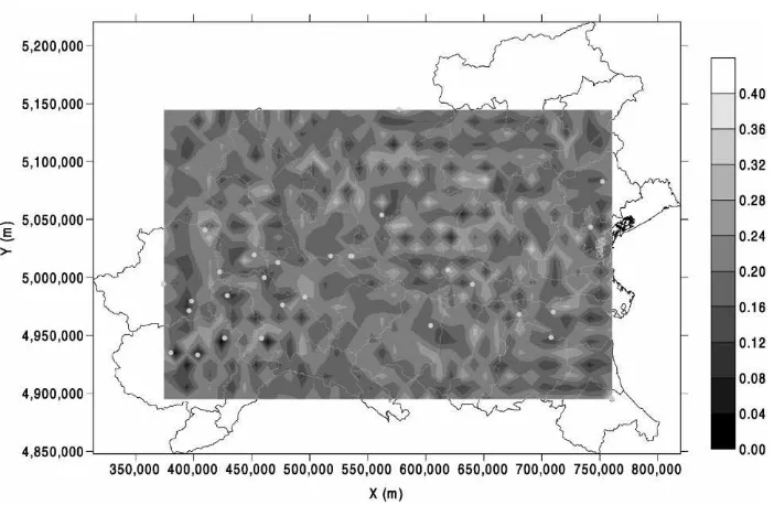
Fig. 4. ‘Simulate the inputs, calculate later’ procedure: map of the average of 20 atmospheric transmissivities calculated on the basis of stochastically simulated inputs (with simulated annealing), for day of year (Day 36).
grid of 40×26 nodes (Fig. 3). The maps give an im-pression of the actually occurring spatial variability of model output. They clearly show low variability as the pattern of calculated atmospheric transmissivity is almost the same for each realisation.
As compared to the interpolated map of Day 36 (see Fig. 2) much more detail can be observed, although the general pattern (low values in the south western part) is the same. It shows that input of simulated values into a agricultural model would be a realistic option to include the actually occurring spatial variability.
3.2.4. SC procedure
Again for Day 36, 20 realisations for each input variable were created with simulated annealing. By applying the model to the simulated inputs at grid nodes and averaging the realisations, a rather frag-mented but homogeneous map is obtained (Fig. 4). This is in contrast to more homogeneous maps ob-tained for CS procedure for the same day (Fig. 3). It underlines the high spatial uncertainty of this system where variation of the input variables is such that only an ‘average’ impression is obtained. Much variation that was visible from the CS procedure, such as the
high values in the south-western part of the area, now disappears.
4. Discussion
tem-perature range, regulated by the Tnc parameter. The CI procedure, on the other hand, requires only inter-polation of the calculated variable, hence leading to a lower error. The IC procedure could be applied only if high-quality and reliable spatial and temporal struc-tures are identifiable for model inputs. In particular, data collected at closer locations would be necessary to identify properly the variogram for those distances where interpolation is required.
For simulation procedures, a similar remark applies: SC highlights a high spatial uncertainty of the model, while CS yielded a more robust result.
Different IC procedures could also be tested, in which model inputs (daily temperatures and local pa-rameters) are not interpolated with OK, but are chosen for each site as the values measured at the nearest sta-tion (or as the average of the values measured at the two or three nearest stations). Also, the local param-eters b and Tnc could be estimated with the transfer functions cited above. Finally, the SC procedure could be improved by co-simulating Tmaxand Tmin.
5. Concluding remarks
In this study, the following conclusions are derived: 1. A relatively simple model to calculate atmospheric transmissivity was found that represents a reliable way to estimate global solar radiation.
2. Model inputs and model output show a clear spatial and temporal structure. Interpolation at the scale of northern Italy yields relatively large MSE val-ues, although CI procedures reduced MSE values with 40% as compared to CI procedures. Future developments may focus on transfer functions for estimating site specific parameters as a function of weather patterns and simpler IC procedures by es-timating model inputs with data from the nearest stations.
3. Different simulations of model output showed sim-ilar patterns of spatial variation as those obtained with interpolation, but with higher spatial variation. Simulation of input data followed by model cal-culations only yielded an ‘average’ result, due to the high spatial and temporal variation of the input data.
4. Modern geostatistical space–time procedures are useful to estimate solar radiation at spatial
loca-tions and at times over large areas of land when no observations are available. This allows improved use of water budget and crop productivity models and to assess the error associated to the estimates of evapotranspiration at each location.
Acknowledgements
The following institutes are gratefully acknowled-ged for providing the data used in this study: Servizio Meteo Idrografico — Regione Piemonte, Torino; Ente Regionale di Sviluppo Agricolo della Lombardia, Seg-rate (MI); Ente Nazionale Risi — Centro Ricerche sul Riso, Castello d’Agogna (PV); Ufficio Centrale di Ecologia Agraria, Roma; Istituto di Agronomia, Uni-versità degli Studi, Milano; Istituto Tecnico Agrario ‘C. Gallini’, Voghera (PV); Istituto Sperimentale per le Colture Foraggere, Lodi; Servizio Metereologico Regionale A.R.P.A. Emilia Romagna, Bologna.
Prof. Tommaso Maggiore (Istituto di Agronomia, Università degli Studi, Milano) is kindly acknowl-edged for giving support to this work and for helping in data collection.
Finalised Project PANDA, Subproject 1, Series 2, Paper No. 43. RadEst 2.1 is freely available at the URL: http://www.inea.it/isci/mdon/software/radest/ RE index.htm.
References
Bindi, M., Miglietta, F., 1991. Estimating daily global solar radiation from air temperature and rainfall measurements. Climate Res. 1, 117–124.
Bindi, M., Fibbi, L., Maracchi, G., 1996. A comparative study of radiation estimation methodologies. European Commission, EUR 16429.
Brinsfield, R., Yaramanoglu, M., Wheaton, F., 1984. Ground level solar radiation prediction model including cloud cover effects. Solar Energy 33, 493–499.
Bristow, R.L., Campbell, G.S., 1984. On the relationship between incoming solar radiation and daily maximum and minimum temperature. Agric. For. Meteorol. 31, 159–166.
Deutsch, C.V., Journel, A.G., 1998. GSLIB: Geostatistical Software Library and User’s Guide, 2nd Edition. Oxford University Press, New York.
Donatelli, M., Marletto, V., 1994. Estimating surface solar radiation by means of air temperature, In: Proceedings of the 3rd Congress of the European Society for Agronomy, Padova, Italy, pp. 352–353.
Elizondo, D., Hoogenboom, G., McClendon, R.W., 1994. Development of a neural network to predict daily solar radiation. Agric. For. Meteorol. 71, 115–132.
Hargreaves, G.L., Hargreaves, G.H., Riley, J.P., 1985. Irrigation water requirements for Senegal River Basin. J. Irrig. Drainage Eng. 111, 265–275.
Hodges, T., French, V., LeDuc, S., 1985. Estimating solar radiation for plant simulation models. AgRISTARS Tech. Rep. JSC-20239 YM-15-00403.
Hook, J.E., McClendon, R.W., 1992. Estimation of solar radiation data missing from long-term meteorological records. Agron. J. 88, 739–742.
Hunt, L.A., Kuchar, L., Swanton, C.J., 1998. Estimation of solar radiation for use in crop modelling. Agric. For. Meteorol. 91, 293–300.
Iqbal, M., 1983. An Introduction to Solar Radiation. Academic Press, Toronto, pp. 106–167.
Journel, A.G., Huijbregts, C.J., 1978. Mining Geostatistics. Academic Press, New York.
Kirkpatrick, S., Gelatt, C.D., Vecchi, M.P., 1983. Optimisation by simulated annealing. Science 220, 671–680.
Loague, K., Green, R.E., 1991. Statistical and graphical methods for evaluating solute transport models: overview and application. J. Contam. Hydrol. 7, 51–73.
McCaskill, M.R., 1990. Prediction of solar radiation from rainy day information using regionally stable coefficients. Agric. For. Meteorol. 51, 247–255.
Nikolov, N.T., Zeller, K.F., 1992. A solar radiation algorithm for ecosystem dynamic models. Ecol. Model. 61, 149–168. Reddy, S.J., 1987. The estimation of global solar radiation and
evaporation through precipitation — a note. Solar Energy 38, 97–104.
Stein, A., Staritsky, I.G., Bouma, J., van Eijnsbergen, A.C., Bregt, A.K., 1991. Simulation of moisture deficits and areal inter-polation by universal cokriging. Water Resour. Res. 27, 1963– 1973.