Full Terms & Conditions of access and use can be found at
http://www.tandfonline.com/action/journalInformation?journalCode=ubes20
Download by: [Universitas Maritim Raja Ali Haji] Date: 11 January 2016, At: 22:38
Journal of Business & Economic Statistics
ISSN: 0735-0015 (Print) 1537-2707 (Online) Journal homepage: http://www.tandfonline.com/loi/ubes20
Habit Persistence and Teen Sex: Could Increased
Access to Contraception Have Unintended
Consequences for Teen Pregnancies?
Peter Arcidiacono , Ahmed Khwaja & Lijing Ouyang
To cite this article: Peter Arcidiacono , Ahmed Khwaja & Lijing Ouyang (2012) Habit Persistence and Teen Sex: Could Increased Access to Contraception Have Unintended Consequences for Teen Pregnancies?, Journal of Business & Economic Statistics, 30:2, 312-325, DOI: 10.1080/07350015.2011.652052
To link to this article: http://dx.doi.org/10.1080/07350015.2011.652052
Published online: 24 May 2012.
Submit your article to this journal
Article views: 704
Habit Persistence and Teen Sex: Could
Increased Access to Contraception Have
Unintended Consequences for Teen
Pregnancies?
Peter A
RCIDIACONODepartment of Economics, Duke University, Durham, NC 27708, and NBER, Cambridge, MA 02138 ([email protected])
Ahmed K
HWAJASchool of Management, Yale University, New Haven, CT 06510 ([email protected])
Lijing O
UYANGCenters for Disease Control and Prevention, Atlanta, GA 30329 ([email protected])
We develop a dynamic discrete-choice model of teen sex and pregnancy that incorporates habit persistence. Habit persistence has two sources here. The first is a “fixed cost” of having sex, which relates to a moral or psychological barrier that has been crossed the first time one has sex. The second is a “transition cost,” whereby once a particular relationship has progressed to sex, it is difficult to move back. We estimate significant habit persistence in teen sex, implying that the long-run effects of contraception policy may be different from their short-run counterparts, especially if the failure rate of contraception is sufficiently large. Programs that increase access to contraception are found to decrease teen pregnancies in the short run but increase them in the long run.
KEY WORDS: Contraceptive policy; Dynamic discrete choice.
1. INTRODUCTION
Teenage pregnancy rates, although steadily declining since 1990, are still very high in the United States, with 83.6 pregnan-cies per 1000 teenage women in 2000 (The Alan Guttmacher Institute2004). This rate is substantially higher than in Canada and Western Europe (Singh and Darroch 2000). Furstenberg (1998) argued that the higher rate in the United States is in part due to the lack of availability of contraception compared with Western Europe. On the other hand, it may be argued that in-creased availability of contraceptives will decrease the rate of unprotected sexandlead some individuals to choose sex when they otherwise would have abstained due to the lower risk of pregnancy because of lowered costs of contraception.
Previous research has shown that regulations and the avail-ability of contraception affect sexual behavior. Research based on aggregate data has found that restrictions on Medicaid fund-ing of abortions or access to clinics reduced the number of adolescent abortions but either had no effect or reduced the number of teen births (e.g., Kane and Staiger 1996; Levine, Trainor, and Zimmerman1996). For abortions to fall with no effect on teen births, there must be a strong behavioral response in sexual activity. Using data from the United Kingdom, Paton (2002) found no evidence that nearness to family planning clin-ics reduced either the pregnancy rate or the abortion rate, with some evidence that family clinics increased the pregnancy rate, while Girma and Paton (2006) found no effect of the availability of emergency contraceptives on teen pregnancies.
Should contraception become more available, some individ-uals could switch from unprotected sex to protected sex, which
could potentially lower the number of teen pregnancies; on the other hand, some individuals could move from abstaining to pro-tected sex, which could increase the number of teen pregnancies through the potential for contraception failure. Hence, the net effect of increased access to contraception on the teen preg-nancy rate would depend on the relative magnitude of these two changes. Moreover, the effects of contraception policy may dif-fer between the long and the short run if there is habit persistence in teen sexual behavior. While habit persistence is generally as-sociated with addictive goods, such as alcohol or cigarettes, it can result from other sources as well. For example, if there is a moral or psychological barrier that is crossed the first time one has sex (a fixed cost), once an individual has sex, he/she will be more likely to have sex in the future. Evidence, even if anecdotal, that a fixed cost to sex may exist is to be found in the growth of social movements for “virginity pledges,” where promises are made to wait until marriage before having sex. Virginity movements have been associated with significant de-creases in teen sex and pregnancy rates, particularly for those under the age of 18 (Bearman and Br¨uckner1997). The impor-tance of virginity is implicitly stressed by much of the sociolog-ical literature on adolescent sex through the attention paid to the time of first intercourse (see Zelnik and Shaw1983; Zabinet al.
© 2012American Statistical Association Journal of Business & Economic Statistics
April 2012, Vol. 30, No. 2 DOI:10.1080/07350015.2011.652052
312
1986; Furstenberg, Brooks-Gunn, and Morgan1987; Day1992; Widmer 1997). This emphasis on virginity suggests that the costs to abstaining from sex are higher for those who have been sexually active in the past.
In this article, we examine the difference between the short-and the long-run effects of contraception policy that may arise due to the presence of habit persistence in sexual activity. We estimate a dynamic model of sex and fertility for teenage women that allows for habit persistence in both the choice to have sex and the choice to contracept. In each year, individuals decide whether to be sexually active, and if so, whether to use con-traception that requires advanced planning (e.g., the pill) or to use contraception that can be implemented at the time of the act itself (e.g., condoms). Should an individual choose to engage in sex, she becomes pregnant with a probability that depends upon the choice of contraception. As in Hotz and Miller (1993) and Carro and Mira (2006), contraception will reduce, but not eliminate, pregnancy risk. We use the model estimates to fore-cast the short-run and long-run effects of increased access to contraception on the rates of teen sex and pregnancy.
The estimates of the model reveal strong habit persistence in teen sexual behavior. These effects are so strong that policies which increase access to certain types of contraception, such as condoms, while lowering teen pregnancy rates in the short run may raise teen pregnancy rates in the long run. Consider a 16 year old exposed to a policy that increases access to contra-ception,ceteris paribus. Our counterfactual simulations reveal that if the policy is a surprise, then the impact of the program on the individual’s pregnancy rate at age 16 is small. However, a 14 year old exposed to the same policy from the age of 14 through 16 will actually have a higher probability of becoming pregnant at age 16. The differences in the long- and short-run effects are driven by habit persistence, especially if the failure rate of contraception is sufficiently large. Individuals who are 16 at the time the policy was implemented have already established certain sexual behaviors. Individuals exposed to the policy from age 14 are more sexually active due to “moral hazard” arising from the lower contraception costs (which lowers the risks of pregnancy). This increased sexual activity is reenforcing due to habit persistence and results in higher long-run pregnancy rates. Thus, our results imply that well-intentioned policies regarding teen access to contraception can have unintended consequences in the presence of habit persistence. At the same time, while increasing access to contraception may be counterproductive, reducing contraception failure rates are not. Namely, when con-traception becomes more effective, our results suggest falls in teen pregnancy rates.
Previous dynamic models of fertility decisions have not fo-cused on the persistence of sexual behavior (e.g., Wolpin 1984; Rosensweig and Shultz 1985; Hotz and Miller 1998, 1993). This is primarily because these studies focus on married cou-ples and the optimal spacing of children; the act of sex itself is taken as given. Models of teen behavior have not focused on the dynamics of sex, in part because of inadequate data. Indeed, the two studies perhaps most related to our own, Lundberg and Plotnik (1995) and Oettinger (1999), used an earlier version of our dataset, which only asked at what age the individual first had sex; year-by-year questions on sexual behavior were not asked.
Lundberg and Plotnick (1995) estimated a sequence of choices in a static context using data from the 1979 National Longitudinal Survey of Youth (NLSY79). They estimated a nested logit model where the sequence of decisions is whether to have a premarital pregnancy, conditional on pregnancy; whether to have an abortion, conditional on not having an abortion; or whether to get married. Lundberg and Plotnick (1995) found that the behavior of whites responds to the incentives of state welfare, abortion, and family planning policies. While we do not model the decision to marry or abort, we do model the choice to have sex and the choice of contraception, and we explicitly account for the dynamics of the decisions.
Oettinger (1999) is one of the few studies in the economics literature to actually examine the decision to have sex as opposed to fertility outcomes. His work also looks at fertility outcomes as well, but does not link the model of fertility to the model of sex. He estimated a hazard model of the time to first sex and the time to first pregnancy using the NLSY79. Persistence in sexual activity, however, could not be taken into account because the survey only asked when the respondent first engaged in sexual activity.
2. MODEL AND ESTIMATION
What distinguishes our work from much of the previous liter-ature is that we do not model fertility as a single choice but as a sequence of choices integrated with uncertainty about pregnancy outcomes. Similar to Hotz and Miller (1998,1993), individuals make decisions regarding sex, knowing that there is some prob-ability of becoming pregnant, with the probprob-ability being lower if contraceptives are used. Individuals may still engage in unpro-tected sex even thoughex post, they may regret the decision if they become pregnant. This can still be consistent with a rational expectations framework. The key is that given the probability of getting pregnant without contraception, the expected utility was still higher for having unprotected sex. Hence, the flow utility of having sex without contraception compensated the individual for the increased probability of becoming pregnant. We first dis-cuss the model without including unobserved heterogeneity and then follow with how unobserved heterogeneity is incorporated.
2.1 Base Model
We propose a dynamic discrete choice model of sex and contraception decisions. Throughout the model, we want to dis-tinguish “flow utility,” utility in the period, from the full con-sequences of having sex, which include the utility of various pregnancy outcomes. Although decisions with regard to sex are joint decisions, since women have to bear the consequences of a pregnancy through carrying the child and have the exclu-sive right to abort the child, we model the decisions from the perspective of the woman.
In each period of T periods, women choose whether to en-gage in sexual activity. Those who enen-gage in sex must also decide whether to contracept, and if so, what type of contra-ception to use. We distinguish between two types of contracep-tion: scheduled contraception, which requires advanced plan-ning, such as the pill, andepisode-specific contraception, where the choice to use it can be postponed until the act itself. Define
ct as the sex and contraception combination chosen at timet
NC if sex but no contraception
EC if sex with episode-specific contraception SC if sex with scheduled contraception
(1)
Conditional on having sex, individuals also choose among dis-crete levels of their sexual activity. In particular, we assume that the level of sexual activity,lt, takes on one of three values: low,
medium, or high,{L, M, H}. As we discuss in Section 3, these levels correspond to 1–10 times since the date of last interview, 11–50 times, and 51 or more times.
Individuals receive flow utility from having sex that may vary across observable characteristics, such as the family en-vironment. The flow utility may also depend upon past sexual decisions. We allow there to be both a fixed and a transition cost for sex itself, as well as fixed and transition costs for the two types of contraception. The fixed and transition costs for sex are included to capture a moral or psychological barrier as-sociated with losing one’s virginity (the fixed cost) or through having sex the first time in a particular relationship (the tran-sition cost). With regard to contraception, in addition to a per-period cost to using it, there may be a fixed cost to learning or acquiring particular contraception, and it may also be easier to access particular forms of contraception if they were used recently. Letsf t represent the possible fixed cost states andslt
the lagged choices, which are over the same set asct. Define
sf t as:
NS if never had sex in the past
NC if had sex in the past but never used contraception
EC if had sex in the past but only used episode-specific contraception or no contraception
SC if had sex in the past but only used scheduled contraception or no contraception
BC if had sex in the past and have used both scheduled and episode-specific contraception Note that these fixed and transition costs depend upon whether the individual engaged in particular acts, not how often.
The utility of sex may also be a function of the family envi-ronment (e.g., mother works, two-parent family, religion). We denote these variables as sxt. Normalizing the flow utility of
abstaining to zero, the base utilities of engaging in sexual ac-tivity (regardless of level) without contraception, with episode-specific contraception, and with scheduled contraception are specified as follows:
Note that the coefficients on sxt are common across the sex
choices. Similarly, the fixed and transition costs for sex itself does not vary across the contraception choices.
The total flow utility depends on the choice of the level of sexual activity, lt, age, sat, and preference shocks for
partic-ular contraception and sex-level combinations, ǫt(ct, lt). We
assume that theǫ’s are distributed Type I extreme value and iid across time and choices. More general correlation struc-tures are possible using a GEV (generalized extreme value) framework (e.g., Khwaja2001; Arcidiacono2005). We exper-imented with more flexible correlation structures and were un-able to reject the Type I extreme value assumption. Further, to ensure that we are truly picking up habit persistence, we allow for the utility of each of the possible choices to de-pend flexibly on age. We must therefore set the discount fac-tor, setting β=0.9, though using different values for β did not qualitatively change our results. We use separate age dum-mies for each of the sex and contraception choices,α6(ct, sat),
as well as separate age dummies for each of the levels of sexual activity,α7(lt, sat). Finally, we have separate dummies
for each contraception choice and sex combination,α8(ct, lt).
The flow utility for a particular choicect andlt is then given
by:
U(ct, lt, st, ǫt)=u(ct, st)+α6(ct, sat)+α7(lt, sat)
+α8(ct, lt)+ǫt(ct, lt). (5)
Those who engage in sex weigh the flow utility of sex against the probability and consequences of becoming pregnant. Denote
yt =1 if a pregnancy results from a sex act att. Conditional on
having sex, the probability of becoming pregnant will depend upon age, the choice of contraception, and the level of sexual activity. We assume that the probability of becoming pregnant follows a logit form:
Pr(yt|ct, lt, sat)=pclt
= exp(satγ0+γ(ct)+γ(lt)+(ct=NC)sat)γ1
1+exp(satγ0+γ(ct)+γ(lt)+(ct =NC)satγ1)
. (6)
The γc’s refer to indicator variables for each of the possible
contraception choices (no contraception, episode-specific, or scheduled). We assume that individuals know these probabilities when they make their sex decisions.
Given that the decision as to whether to abort or give birth is often very traumatic, and given limited data on abortions, we do not model the abortion decision. Rather, we model the lifetime utility after pregnancy using a terminal value function. The terminal value function,Vpt, flexibly maps the states attthat
we expect to affect the lifetime utility of a pregnancy,spt, into
discounted present value utility. The next section describes the variables that are used as input into the terminal value function. Examples of variables that will affect this terminal utility but not the flow utility of having sex are ability measures and family income, as the opportunity cost of a child will be higher for
those who have better expected labor market outcomes. Note that treating pregnancy as terminal state in no way diminishes the importance of future labor market outcomes when making sexual decisions. Individuals may recognize how pregnancies affect their educational paths and future work profiles. Indeed, as the estimation reveals, the human capital measures in the terminal value function play a significant role in sexual activity choices.
In addition to uncertainty regarding future pregnancy out-comes and unobservable preferences, individuals also face un-certainty regarding the state variables themselves. We assume that individuals know the stochastic processes governing the transitions of the demographic variables, and these transitions do not depend upon decisions made by the individual regarding their sexual behavior. Since the transitions on the demographic variables are not the focus of the analysis, we discuss the es-timation of the transitions of these variables in the Appendix. While uncertainty also exists due to the probability of contract-ing a sexually transmitted disease (STD), our dataset includes no information on STDs.
The transition of sexual histories is completely determined by the individuals’ choices. Letst denote the full set of state
vari-ables, including the state variables that affect sex, the transitions on the demographics, the cost of pregnancy, and the probability of pregnancy, We then specify the probability of moving from statest tost+1asq(st+1|st, ct), implying thatst−1 only affects
st+1 through st andct. Note that the conditioning onct only
matters through the sexual histories.
Since we are only interested in teen sexual behavior, we also assign a terminal value for individuals who arrive to age 19 without becoming pregnant. Normalizations must be made to identify the model. We normalize the utility of mak-ing it to age 20 (T + 1) without a pregnancy to zero. The conditional value functions at T, v(cT, lT, sT, ǫT), are then
given by
vT(cT, lT, sT, ǫT)=UT(cT, lT, sT, ǫT)+βpclTVpT+1(spT+1),
(7) whereβis the discount factor. The value function at timeTis thenVT(sT, ǫT)=maxcT,lT{vT(cT, lT, sT, ǫT)}.
The conditional valuation functions atT −1 then follow:
vT−1(cT−1, lT−1, sT−1, ǫT−1)
=UT−1(cT−1, lT−1, sT−1, ǫT−1)+βE[pclT−1VpT(spT)
+(1−pclT−1)VT(sT, ǫT)|cT−1, sT−1], (8)
where the expectations are taken over pregnancies and the val-ues of the observed and unobserved state variables. Using back-wards recursion, we can then write the conditional valuation functions at timetas
vt(ct, lt, st, ǫt)=Ut(ct, lt, st, ǫt)+βE[pcltVpt+1(spt+1)
+(1−pclt)Vt+1(st+1, ǫt+1)|ct, st]. (9)
Given the assumptions on the ǫ’s, closed-form solutions for the conditional expectations of future utility exist (Rust
1987). Denotevt(ct, lt, st)=vt(ct, lt, st,0), the conditional
val-uation function net of theǫ’s. We can then write Equation (9) as
whereecis Euler’s constant.
Probabilities of choosing particular sex and contraception combinations then yield multinomial logit probabilities, where instead of the term inside the exponential function being linear in the parameters, it is highly nonlinear. The log-likelihood function is then the sum of three parts:
1. Lc– the log-likelihood of the sex and contraception choices,
2. Ly – the log-likelihood of the pregnancy outcomes, and
3. Ls– the log-likelihood of the transitions on the
demograph-ics.
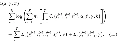
The full log-likelihood function is then:
L(α, γ)= whereLc,Ly, andLsrefer to the log-likelihood contributions of
the sexual activity and contraception decisions, the probability of becoming pregnant, and the transitions on the other state vari-ables for each individualn=1, . . . , N. Since the log-likelihood is additively separable, it is possible to estimate the parameters of the model in stages. In particular, we use maximum likeli-hood to first estimate the pregnancy and transition parameters using onlyLy andLs. Next, taking estimates of the pregnancy
and transition parameters as given, we use maximum likelihood to estimate the utility function parameters usingLc.
Note that the reason why the log-likelihood is additively sep-arable is that we have assumed that the unobserved preferences for sex and contraception are independent of the errors in the probability of becoming pregnant. Hence,
Lc
There may, however, still be unobservable preferences for having sex. Not controlling for unobserved heterogeneity may attribute too much sexual activity to habit persistence. To ac-count for unobserved preferences, we estimate the model us-ing mixture distributions to allow for unobserved heterogeneity in the taste for sex. Mixture distributions can be used to over-come this problem and control for “dynamic selection” (e.g., see Keane and Wolpin1997; Cameron and Heckman1998,2001;
Eckstein and Wolpin1999; Gilleskie and Strumpf2005). In their analysis of married couples, Carro and Mira (2006) modeled the unobserved heterogeneity on pregnancy probabilities rather than sex. We assume that there areKtypes of people, withπkbeing
the population probability of being the kth type. Preferences are common across types and types are known to the individu-als. We assume that conditional on observed characteristics and one’s unobserved type, the unobserved preferences are serially uncorrelated. Hence, the flow payoffs for choices that entail sex have an additional type-specific intercept,α9k, withα9k
normal-ized to zero. Hence, type is conditioned on in the conditional valuation functions, vt(ct, lt, st, k, ǫt), the ex-antevalue
func-tions, Vt(st, k), and flow payoff functions, Ut(ct, lt, st, k, ǫt).
The probability of choosing the combination{ct, lt}conditional
on the observed states and being thekth type is then Pr(ct, lt|st, k)
Treating type as a random effect, it is possible to integrate out the probability of being a particular type. The log-likelihood function is then
where theL’s are the likelihoods rather than the log-likelihoods,
and theπ’s are the population probabilities of being a particular type. In principle, these population probabilities can vary with state variables, as in Keane and Wolpin (1997, 2000, 2001) and Arcidiacono, Sieg, and Sloan (2007). This is done to account for initial conditions, something that is unnecessary as we have the full sex history. We assume that the probability of a pregnancy, conditional on sexual behavior as well as the other transition processes, does not depend upon type (we test this assumption in Section 4). Hence, we can rewrite the log-likelihood as
L(α, γ , π)
Estimation can again proceed in stages. As before, we first estimate the probability of becoming pregnant, conditional on the choice of sexual activity as well as the transitions on the demographic variables. Taking these parameters as given, we estimate the parameters of the utility function.
3. DATA
We use the 1997 National Longitudinal Survey of Youth (NLSY97) to estimate the model. The NLSY97 data contain
surveys of youths born during the years 1980–1984. The first survey was conducted in 1997, when the individuals were be-tween the ages of 12 and 16. Participants are interviewed roughly each year, with blacks and Hispanics oversampled.
In each wave, those surveyed by the NLSY97 answer ques-tions about their sexual activity. To accommodate the model in the previous section, we discretize sexual frequencies into three categories: having sex 1–10 times since the date of last interview, 11–50 times, and more than 50 times. Conditional on being sexually active in a particular year, 45%, 34%, and 21% were in each of the groups, respectively. We examine how discretizing the data in this way affects our results in Section 4. The participants were also asked what percentage of the time they used contraception and what their primary form of con-traception was. Almost 59% of the participants reported using birth control every time they had sexual intercourse. Note that this does not include those who reported withdrawal or rhythm as their method of birth control. We classify those who use contraception less than 100% of the time under the unprotected (no contraception) category. Those individuals who reported using contraception every time but whose primary method of birth control was withdrawal or the rhythm method were clas-sified as unprotected as well. Episode-specific contraception was defined as condoms, foam, jelly, sponges, and diaphragm. Scheduled contraception was defined as the pill, intrauterine de-vices (IUDs), Norplant, Depo-Provera, and injectables. In ear-lier waves, individuals were asked what fraction of the time they used birth control and, if they were protected, what the primary method of birth control was. In later waves, the in-dividuals were first asked what percentage of the time a con-dom was used when they had sex. They were also asked what percentage of the time birth control was used as well as the primary birth control method besides a condom. If the woman reported using a condom 100% of the time, then the birth control method was classified as episode-specific. If all the acts were protected but a condom was used less than 100% of the time, we used the primary method besides a condom to determine whether to classify the birth control as episode-specific or scheduled.
We only use continuous sex histories beginning from age 14. For example, if an individual is 14 in wave 1 and answers the sex questions in waves 1 and 2 but not in wave 3, no survey answers after wave 2 would be used regardless of whether or not answers were given in waves 4 and 5. For more detailed descriptive statistics on the sex rates and the use of contraception, see Walker (2003). Finally, we only keep those individuals who had not experienced a pregnancy as a result of sex from a previous survey wave.
Table 1shows the sex patterns for women who answered the questions on whether they had sexual intercourse in the first four waves of the survey and who were between the ages 14 and 16 in wave 1. The first set of rows shows patterns of sexual behavior where the individual has had sex in at least two waves but, once they started having sex, continued to have sex from then on. The second set of rows show histories where after the individual had started having sex, at least one break in sexual activity occurred. The final set of rows are histories for those who either abstained until the final wave or abstained in every wave. Comparing the first set of rows, where no break in sexual activity occurs, with the second set of rows shows that in general, once one is sexually
Table 1. Persistence in female sexual activitya
Age in 1997
Sex in 1997 Sex in 1998 Sex in 1999 Sex in 2000 14 15 16 Overall
No No Yes Yes 13.3% 12.4% 11.9% 12.5%
No Yes Yes Yes 15.5% 18.0% 21.0% 18.4%
Yes Yes Yes Yes 8.8% 16.4% 27.1% 18.0%
Yes No No No 0.4% 0.6% 0.5% 0.5%
No Yes No No 0.4% 1.2% 0.9% 0.9%
No No Yes No 0.9% 1.8% 1.9% 1.6%
Yes Yes No No 0.2% 0.5% 0.9% 0.6%
No Yes No Yes 3.8% 2.3% 1.9% 2.6%
No Yes Yes No 0.4% 0.6% 1.4% 0.8%
Yes No No Yes 0.2% 0.8% 0.4% 0.5%
Yes No Yes No 0.0% 0.3% 0.4% 0.3%
Yes No Yes Yes 0.4% 1.8% 1.2% 1.2%
Yes Yes No Yes 0.7% 1.2% 1.1% 1.0%
Yes Yes Yes No 0.0% 0.5% 1.4% 0.7%
No No No Yes 13.5% 11.5% 8.6% 11.0%
No No No No 41.3% 30.1% 19.4% 29.4%
aAll females who had valid answers for the sex questions in first four waves. Sample sizes are 498, 727, and 640 for ages 14, 15, and 16, respectively.
active, she remains so from that point forward. Similar patterns hold for males as well, with slightly more males having breaks in their sexual behavior, suggesting women may be the ones dictating whether sex occurs.
Note that person-specific effects cannot be completely driving the persistence. For example, consider an individual who had sex in 1997 but not in 1998. This individual is considerablyless
likely to have sex in 1999 than someone who had sex in 1998 but not in 1997. Having sex in one year and not the next is rare. In fact, the least likely outcome for all ages was a pattern of two stops in sexual activity: having sex, then not; then having
sex, then not. The patterns in the data then suggest that there may be a fixed cost (a moral or psychological barrier that has been crossed) and a transition cost (which may be relationship-specific).
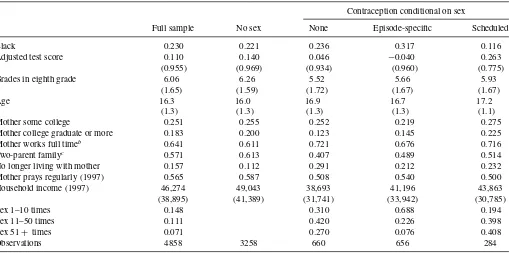
Means conditional on the choice of sex and contraception type are given inTable 2using the first five waves of the survey. Only individuals 14 and older were asked the sex questions, while only individuals 14 and younger in 1997 were asked about parental religious practices, limiting our sample sizes. We also eliminate all individuals who did not report a family income in wave 1. A little over 13% of the sample was classified as unprotected,
Table 2. Means conditional on sex and contraception choicesa
Contraception conditional on sex
Full sample No sex None Episode-specific Scheduled
Black 0.230 0.221 0.236 0.317 0.116
Adjusted test score 0.110 0.140 0.046 −0.040 0.263
(0.955) (0.969) (0.934) (0.960) (0.775)
Grades in eighth grade 6.06 6.26 5.52 5.66 5.93
(1.65) (1.59) (1.72) (1.67) (1.67)
Age 16.3 16.0 16.9 16.7 17.2
(1.3) (1.3) (1.3) (1.3) (1.1)
Mother some college 0.251 0.255 0.252 0.219 0.275
Mother college graduate or more 0.183 0.200 0.123 0.145 0.225
Mother works full timeb 0.641 0.611 0.721 0.676 0.716
Two-parent familyc 0.571 0.613 0.407 0.489 0.514
No longer living with mother 0.157 0.112 0.291 0.212 0.232
Mother prays regularly (1997) 0.565 0.587 0.508 0.540 0.500
Household income (1997) 46,274 49,043 38,693 41,196 43,863
(38,895) (41,389) (31,741) (33,942) (30,785)
Sex 1–10 times 0.148 0.310 0.688 0.194
Sex 11–50 times 0.111 0.420 0.226 0.398
Sex 51+ times 0.071 0.270 0.076 0.408
Observations 4858 3258 660 656 284
aStandard deviations in parentheses.
bConditional on living with one’s biological mother and after wave 1. In wave 1, no distinction was made between part-time and full-time work. cConditional on living with one’s biological mother. No updated information is available on these variables when the individual leaves home.
with 13% and 6% using episode-specific and scheduled contra-ception, respectively. Those who engage in sex tend to be older, particularly those who choose scheduled contraception.
With the exception of the level of sexual activity, the variables listed either affect the flow utility directly or affect decisions through the terminal value function. All independent variables are taken from wave 1 of the survey, with the exception of mother working, two-parent family, and whether the individuals were living with their biological mother. The mother working variable takes on a value of 1 if the mother works full time. In wave 1, we do not observe whether the mother worked full time or part time. For wave 1, we classify a mother as working full time if she also worked full time in wave 2. For those who did not work full time in wave 2 but reported working full time in wave 1, we set the probability of working full time in wave 1 to match the transitions from work to not work, and work to work in the future waves. Two-parent family refers to the family structure where the teen lives with both biological parents. While coming from a two-parent family is associated with less sex, having a working mother or no longer living with one’s biological mother is associated with higher sexual activity.
Characteristics of the mother and the household itself are highly correlated with sexual activity. Having a college-educated mother makes abstaining more likely, but also more likely that the individual will choose scheduled contraception. Having a mother who prays more than once a day is associated with abstaining, as is coming from a two-parent family, higher test scores, and higher grades. Higher test scores and grades are also associated with choosing scheduled contraception over the other contraception categories. The test score used was the adjusted PIAT math score. The mean is above zero in the pop-ulation because women score higher than men. The grade cate-gories were: 1 = mostly below D’s, 2 = mostly D’s 3 = about half C’s and half D’s, 4 = mostly C’s, 5 = about half B’s and half C’s, 6 = mostly B’s, 7 = about half A’s and B’s, and 8 = mostly A’s.
Those who use scheduled contraception have sex more of-ten than those in the other contraception categories. Episode-specific contraception is associated with the least frequency conditional on being sexually active. This may be in part driven by our requirement of having individuals use protection 100% of the time to be counted as protected. We investigate the ro-bustness of our results to this assumption later in the article.
The NLSY97 contains detailed information on the timing of births, abortions, and miscarriages. For the pregnancy data, we date all births, abortions, and miscarriages back to when the sex act would have taken place. A birth reported in wave 2 may have resulted from intercourse in either wave 1 or wave 2. To determine whether pregnancy resulted from sex in wave 1 or wave 2, the date a birth takes place is dated back nine months. This latter date is then linked to the sex decisions for the relevant wave. Similarly, the NLSY97 reports the date of miscarriages and abortions as well as how far along the pregnancy was at the time of the miscarriage or abortion. Pregnancies are then the sum of births, miscarriages, and abortions.
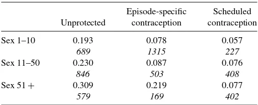
Table 3presents pregnancy probabilities, given the choice of contraception and the level of sexual activity. Because there are so few variables used here and since by assumption the preg-nancy parameters can be estimated outside of the model, we are able to use a much larger sample. The overall pregnancy rate in
Table 3. Probability of becoming pregnant conditional on choice of contraception and level of sexual activitya
Episode-specific Scheduled
Unprotected contraception contraception
Sex 1–10 0.193 0.078 0.057
689 1315 227
Sex 11–50 0.230 0.087 0.076
846 503 408
Sex 51+ 0.309 0.219 0.077
579 169 402
aNumber of observations in italics. Sample includes all females between the ages of 14 and
19 who had sex in waves 1–5. All pregnancies are dated back to the sex decisions in these waves. The sample also include pregnancies reported in wave 6 that resulted from sex acts in wave 5.
the sample is 15% for those who are sexually active. The level of sexual activity strongly correlates with the probability of a preg-nancy. For those who do not report using contraception 100% of the time, the probability of becoming pregnant increases from less than 20% to over 30% as we move from the lowest level of sexual activity to the highest.
Pregnancy rates are much lower if the individual reports using contraception 100% of the time. Although both methods result in much lower pregnancy rates than those who are not protected, scheduled contraception is significantly more effective, partic-ularly in the highest level of sexual activity. We also considered cutoffs lower than 100% to qualify as protected. Although one would expect pregnancy rates to substantially increase for the unprotected group if a lower cutoff is used, using a cutoff of 75% protected has little effect on the average pregnancy probabili-ties for those classified as unprotected. Namely, the pregnancy rates were 18%, 26%, and 30% for the three levels of sexual activity, respectively. In contrast, steep increases in pregnancy probabilities were seen for those using episode-specific contra-ception, with the corresponding pregnancy rates rising to 10%, 16%, and 28%, respectively. This suggests that the pregnancy rates for those who reported using contraception almost all the time are more similar to the rates for those who reported using little contraception than for those who used contraception 100% of the time.
These pregnancy rates may seem high. However, the fact that such high pregnancy rates exist conditional on reported 100% protection is consistent with the medical literature. Black et al. (2010) stated that women in the United States report that 50% of unintended pregnancies are the result of contraceptive failure, with the corresponding number in France being 65%. Trussell’s (2004) review article, where the samples studied are typically older than the ones in our data, found that typical use of male condoms resulted in pregnancy rates of 15%, while if condoms had been used correctly, the rate would have been 2%. Similar to the data here, methods such as the pill are more effective than condoms, both when used correctly and under typical use. Pregnancy rates under typical use for the pill are 8%.
4. RESULTS
We now proceed to the estimates of the model, beginning with the pregnancy parameters. Estimates of the transition
Table 4. Logit estimates of the probability of becoming pregnanta
Coefficient Std. error
Sex 11–50 0.2479 (0.1005)
Sex 50+ 0.6943 (0.1101)
Episode-specific −0.6688 (0.2258)
Scheduled −1.1497 (0.2679)
Age 0.0246 (0.0405)
Contraception×age −0.0933 (0.0652)
Intercept −1.8873 (0.6924)
Observations 5136
aSample includes all females between the ages of 14 and 19 who had sex in waves 1–5. All
pregnancies are dated back to the sex decisions in these waves. The sample also include pregnancies reported in wave 6 that resulted from sex acts in wave 5.
parameters on family status, mother working, and living with one’s biological mother are reported in the Appendix. Recall that the pregnancy parameters are only estimated for those who chose to engage in sexual intercourse.Table 4presents the logit estimates of the probability of a pregnancy. As expected, higher levels of sexual activity are associated with higher probabilities of a pregnancy, while contraception is associated with lower pregnancy probabilities. Individuals become better at using con-traception with age, though the coefficient is not statistically significant.
Adding the number of times an individual had sex did not improve the fit of the model, supporting the conditional inde-pendence assumption. The coefficient on the number of times was small and insignificant, suggesting that we are losing lit-tle by discretizing sexual activity. Further, we tested whether lagged sexual frequency and lagged contraception choice af-fected the probability of becoming pregnant as this would be suggestive that unobserved heterogeneity was also important in pregnancy probabilities. Although lagged sexual frequency was statistically significant, the joint test of the additional lagged variables was rejected at the 95% level. Further, the statisti-cal significance of the lagged sexual frequency was driven by 19 year olds; focusing on those below 18 and younger shrunk the coefficient by 50% and was statistically insignificant.
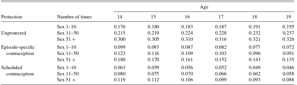
To get a sense of the magnitudes of these effects,Table 5
shows the estimated pregnancy probabilities conditional on age, contraception choice, and level of sexual activity. Increased sex-ual activity increases pregnancy rates, particularly when
contra-ception is not used. A 16 year old moving from the lowest level of sexual activity to the highest sees her probability of becoming pregnant increase by 13 percentage points if unprotected, a little over 7 percentage points if using episode-specific contraception, and by 5 percentage points if using scheduled contraception. Un-protected sex results in pregnancy rates that are 1.5–2.5 times higher than protected sex using episode-specific contraception, and 2.5–4.0 times higher than protected sex using scheduled contraception. These differences may seem small but recall that an individual was classified as having protected sex only if the he/she reported using contraception 100% of the time. The un-protected category then includes individuals who often used protection but did not report using contraception every time. The lower pregnancy rates associated with contraception grow with the individual’s age as the individual learns how to use the contraception correctly.
The parameters characterizing the flow utility of sex are given inTable 6. The first set of rows shows the coefficients on the demographic characteristics. Having a mother who prays reg-ularly and coming from a two-parent family both lowers the utility associated with sex relative to abstinence. In contrast, having a mother who works or not living with one’s biolog-ical mother positively affects the utility associated with sex. Mother’s education has no effect on utility associated with sex, but has a substantial effect on sex choices through the terminal value function.
The specification and coefficient estimates of the terminal value function are reported in the Appendix. What can be seen from those estimates is that pregnancy costs are higher when individual’s mother is college-educated. Due to the nonlinear portions, the other effects are less easy to see, but variables associated with higher human capital (grades, test scores, family income), and therefore greater labor market rewards, increase pregnancy costs as well.
We parameterized the unobserved preferences for sex using a two-type mixture distribution. The second type, which makes up a little less than a quarter of the population, is substantially less likely to have sex than the first type. We experimented with more types but the results consistently yielded estimates such that additional types were indistinguishable from the first two types.
The final set of rows show the persistence parameters. For both contraception choices, we see no transition costs. How-ever, the fixed costs of scheduled contraception is quite large.
Table 5. Estimated pregnancy probabilities
Age
Protection Number of times 14 15 16 17 18 19
Sex 1–10 0.176 0.180 0.183 0.187 0.191 0.195
Unprotected Sex 11–50 0.215 0.219 0.224 0.228 0.232 0.237
Sex 51+ 0.300 0.305 0.310 0.316 0.321 0.326
Episode-specific Sex 1–10 0.099 0.093 0.087 0.082 0.077 0.072
contraception Sex 11–50 0.123 0.116 0.109 0.103 0.096 0.091
Sex 51+ 0.180 0.170 0.161 0.152 0.143 0.135
Scheduled Sex 1–10 0.063 0.059 0.056 0.052 0.049 0.046
contraception Sex 11–50 0.080 0.075 0.070 0.066 0.062 0.058
Sex 51+ 0.119 0.112 0.106 0.099 0.093 0.088
Table 6. Parameters of the utility functiona
Std.
Variable Coefficient error
Black 0.205 0.120
Mother works full time 0.275 0.085
Two-parent family −0.357 0.092
Flow No longer living with mother 0.230 0.116
utility Mother prays regularly −0.239 0.075
Mother some college −0.048 0.122
Mother college graduate or more 0.115 0.147
Type 2 −1.406 0.403
Sex transition cost −1.551 0.258
Sex fixed cost −0.540 0.172
Habit persistence
Episode-specific contraception transition cost
−0.397 0.216
Episode-specific contraception fixed cost
0.306 0.257
Scheduled contraception transition cost
−0.209 0.298
Scheduled contraception fixed cost
−2.258 0.232
Prob. Type 2 0.234 0.041
Observations 4858
aEstimates from the dynamic discrete choice model on only those who have continuous
sex histories. The discount factor is set at 0.9. The utility function included age interacted with each of the choices, which allows for pregnancy costs and flow tastes for the various choices to vary by age.
There then may be a tradeoff between encouraging the use of the pill versus encouraging the use of condoms. Condoms help prevent STDs, but encouraging individuals to use the pill will make birth control more of a habit. Both fixed and transition costs are significant for sex itself, with the transi-tion cost being approximately three times the fixed cost. Such large effects imply that the long-run effects of contraception
policy on sexual behavior may be different from the short-run effects.
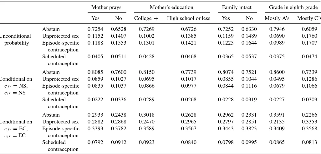
The utility function parameters are difficult to interpret be-cause of the nonlinearities in the choice function. To see how demographic characteristics and habit persistence affect the sex choices, we calculate the probabilities of each of the contracep-tion choices, aggregating over the level of sexual activity, given different demographics and sex histories. In particular, we fore-cast the decisions of 16 year olds, given the characteristics of those who are 14. We then assign the different values for par-ticular demographic characteristics and see how these affect the probability of choosing particular sex options at age 16. Hence, when examining the effects of mother’s education, we assign all individuals to the same level of mother’s education and then repeat with a different level of mother’s education. Results of these simulations are given inTable 7.
The first set of rows gives the unconditional probabilities of sex choices at age 16. Moving from having a mother who does not pray regularly to one who does decreases the probability of having sex by 7 percentage points. Conditional on having sex, unprotected sex is more common for those with mothers who do not pray regularly. Individuals who are more likely to have sex in the future also expect to receive higher benefits from paying the fixed costs associated with contraception. The effect of an intact family is similarly strong—moving from an intact family at age 14 to a single-parent family at age 14 results in a 9 percentage points increase in the probability of having sex at age 16.
Recall that mother’s education had little effect on the pref-erences for sex. However, the effect through the terminal value function is strong. Switching from a mother who has no educa-tion past high school to one with a college educaeduca-tion results in an over 5 percentage point increase in the probability of abstaining. The shift away from sex is particularly strong for unprotected
Table 7. Choice probabilities for those aged 16 under different demographicsa
Mother prays Mother’s education Family intact Grade in eighth grade
Yes No College+ High school or less Yes No Mostly A’s Mostly C’s
Abstain 0.7254 0.6528 0.7269 0.6726 0.7252 0.6330 0.7946 0.6059
Unconditional Unprotected sex 0.1152 0.1407 0.1002 0.1385 0.1159 0.1489 0.0690 0.1760
probability Episode-specific
contraception
0.1188 0.1553 0.1301 0.1421 0.1225 0.1644 0.0989 0.1707
Scheduled contraception
0.0405 0.0511 0.0428 0.0468 0.0365 0.0537 0.0375 0.0474
Abstain 0.8085 0.7600 0.8150 0.7739 0.8074 0.7521 0.8600 0.7339
Conditional on Unprotected sex 0.0859 0.1027 0.0695 0.1017 0.0855 0.1044 0.0495 0.1286
cf c=NS,
c15=NS
Episode-specific contraception
0.0835 0.1037 0.0866 0.0977 0.0844 0.1116 0.0679 0.1066
Scheduled contraception
0.0222 0.0336 0.0289 0.0268 0.0228 0.0319 0.0227 0.0309
Abstain 0.2933 0.2438 0.3018 0.2628 0.2962 0.2331 0.3591 0.2266
Conditional on Unprotected sex 0.2882 0.2868 0.2470 0.2965 0.2797 0.2851 0.2135 0.3353
cf c=EC,
c15=EC
Episode-specific contraception
0.3393 0.3782 0.3589 0.3567 0.3443 0.3823 0.3409 0.3568
Scheduled contraception
0.0792 0.0912 0.0923 0.0840 0.0798 0.0995 0.0865 0.0813
aForecasted from the characteristics of 14 year olds. Effects for intact family and mother works are the effects from having these characteristics at age 14.
Table 8. Comparing model predictions with the dataa
Age=14 Age=15 Age=16 Age=17 Age=18
Probability of: Model Data Model Data Model Data Model Data Model Data
Abstaining 0.8809 0.8745 0.7779 0.8171 0.6830 0.7117 0.5703 0.5942 0.4425 0.4702
Unprotected sex 0.0557 0.0607 0.0878 0.0718 0.1311 0.1198 0.1656 0.1582 0.2397 0.2235
Episode-specific 0.0567 0.0586 0.1160 0.0954 0.1397 0.1286 0.1731 0.1660 0.1910 0.1872
Scheduled 0.0067 0.0063 0.0183 0.0157 0.0462 0.0399 0.0910 0.0817 0.1268 0.119
Sex 1–10 0.0845 0.0879 0.1393 0.1141 0.1838 0.1669 0.1798 0.1702 0.1784 0.1727
Sex 11–50 0.0292 0.0314 0.0581 0.0492 0.0948 0.0879 0.1536 0.1479 0.1998 0.1930
Sex 51+ 0.0054 0.0063 0.0247 0.0197 0.0384 0.0335 0.0963 0.0877 0.1794 0.1640
aModel predictions are calculated using the characteristics of 14 year olds.
sex, with the move away from unprotected sex representing over half of the shift from sex. Grades, which only operate through the terminal value function, have very large effects on the costs of pregnancy, likely due to their association with human capital. Moving from receiving mostly A’s to mostly C’s increases the probability of engaging in sexual activity by almost 19 percent-age points, again with most of the drop coming from unprotected sex.
The next set of rows conditions on history. That is, instead of forecasting what the history will be, given particular de-mographic characteristics, we will instead assume a particular sexual history. The second set of rows assumes a history of no sex, while the third set assumes the person had sex in the pre-vious period (age 15) and used episode-specific contraception. The differences across the second and third set of rows are quite large. While an individual who had an intact family at age 16 would abstain 80% of the time, conditional on abstaining in the past, the probability that a similar individual who had sex using episode-specific contraception in the previous period is 30%. Habit persistence is much more important in determining sexual activity than having a praying mother, an intact family, a mother with a college education, or even grades.
These estimated effects and the policy simulations conducted in the next section are not informative if the model does a poor job of fitting the data. Using the sample of those aged 14, we forecast the sex choices and fertility outcomes and see how well this matches the trends in the data. The model predictions for ages 14 through 18 are shown inTable 8. Although we would expect to match the trends, given the full set of age interactions, we are forecasting ahead with a particular subset of individuals.
While in general, predictions are very close to the data, the model slightly overpredicts sex rates at older ages. Conditional on having sex, the model predicts the level of sexual activity very well.
5. POLICY SIMULATIONS
Given the model matches the predicted choices of sex and contraception use reasonably well, we now turn to policy simu-lations that examine the effects of changes in access to ception for teens. In particular, we forecast the sex and contra-ception decisions and consequent pregnancy outcomes for 16 year olds both when the policy is initially put into place (and thereby surprising the current 16 year olds) and in the next two years after the policy. We use the characteristics of the 14 year olds for the simulations. Hence, in year 3 of the policy, 16 year olds will have been exposed to the policy since they were 14. Our policy simulations are valid under the following assumptions that we have made in our model: (1) unobserved heterogeneity in preferences is time invariant, (2) observed state variables such as age account for any other time variation in preferences, and (3) given the former two assumptions, all preference shocks are independent across time. Given these three assumptions, any remaining structural state dependence is what we label “habit persistence.”
We focus on two hypothetical contraception policies. The first policy simulates the effects of decreasing access to all contra-ception, both episode-specific and scheduled. In this case, the utility of using birth control is decreased (increasing the ef-fective cost), though the utility of sex itself is leftunchanged.
Table 9. Sixteen year old short- and long-run responses to decreasing access to contraceptiona
Unprotected Episode-specific Scheduled
No sex sex contraception contraception Pregnancy
Year 1 3.00% 7.90% −14.57% −18.78% −0.83%
Population Year 2 4.56% 5.18% −17.59% −22.99% −3.73%
Year 3 5.26% 3.77% −18.76% −24.89% −5.14%
Year 1 3.38% 8.97% −13.96% −18.55% 1.31%
Low grades Year 2 5.16% 7.38% −16.38% −22.51% −0.64%
Year 3 6.07% 5.87% −17.00% −24.12% −2.00%
aForecasted from the sample of 14 year olds, assuming the change in policy was a surprise. Percent changes use the forecasts with no policy as the base. To simulate the policy, we lower
the intercept parameters in Equations (3) and (4) by 0.2. We experimented with different values for these changes and the qualitative results remained the same. Low-income forecasts are done only for those individuals who had parents earnings at or below the 25th percentile of the income distribution in the data.
Table 10. Sixteen year old short- and long-run responses to changes in the attractiveness and effectiveness of condomsa
Unprotected Episode-specific Scheduled
No sex sex contraception contraception Pregnancy
Increased Year 1 −2.33% −5.40% 17.64% −7.08% 1.23%
access Year 2 −3.70% −3.43% 21.48% −5.83% 3.70%
Year 3 −4.40% −2.22% 22.92% −4.16% 5.02%
Increased Year 1 −0.26% −0.59% 1.97% −0.90% −2.75%
effectiveness Year 2 −0.42% −0.41% 2.41% −0.61% −2.52%
Year 3 −0.53% −0.23% 2.63% −0.28% −2.33%
Increased both Year 1 −2.65% −6.51% 20.50% −8.21% −2.35%
access and Year 2 −4.32% −4.20% 25.15% −6.45% 0.48%
effectiveness Year 3 −5.16% −2.88% 27.09% −4.67% 1.94%
aForecasted from the sample of 14 year olds whose grades were half B’s and C’s or worse, assuming the change in policy was a surprise. Percent changes use the forecasts with no
policy as the base. For increased access to episode-specific contraception, we increase the intercept parameter in Equation (3) by 0.2, leaving the fixed and transition costs unchanged. We experimented with different values for these changes and the qualitative results remained the same. For increased effectiveness, we increased the efficacy of episode-specific contraception by 10%.
An example of this could be curbing the distribution of contra-ceptives on school premises. The second policy simulates the effects of increases in access to episode-specific contraception and/or increases in the effectiveness of episode-specific contra-ception: ad campaigns that encourage the use of condoms or by making condoms available in school bathrooms, both of which lower the effective costs of using condoms (raising the net utility of episode-specific contraception). Alternatively, sex education classes could lead to increased effectiveness of contraception (lowering pregnancy rates, conditional on contraception use).
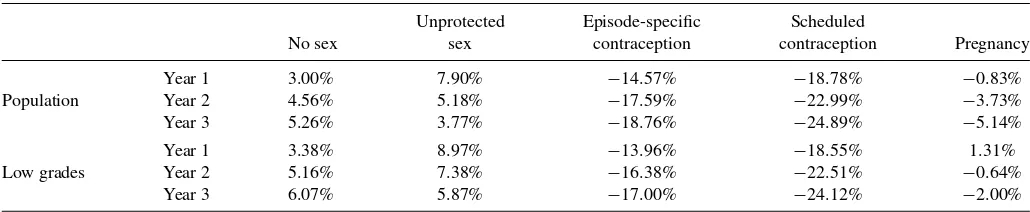
Table 9 shows the effect of the first policy change, decreasing access to contraception, on sexual activity and pregnancy rates, aggregating across the levels of activity, in the first three years of the policy. Each element then gives the percent change in the activity relative to the corresponding activity before the policy change. The first panel of Table 9 reports results for the popula-tion. In year 1 of the policy, decreasing access to contraception results in an almost 8% increase in unprotected sex relative to the pre-policy rate. However, by year 3, the increase is less than 4%. Large shifts are seen away from both contraception meth-ods, and more so with longer exposure to the policy. The shift toward no sex is magnified over time, with a 3% increase relative
to pre-policy in year 1 and an over 5% increase in year 3. Preg-nancy rates drop in all three years of the policy, but are very small in the first year. For the population as a whole, even though rates of unprotected sex increase, the movement away from contra-ception methods that are not fully effective to abstaining results in a drop in pregnancies. The drop in the pregnancy rate relative to the pre-policy pregnancy rate increases with the length of the policy as those who enter age 16 now have different sexual histories.
The effects of the policy may differ depending upon one’s propensity to engage in sexual activity. Namely, if someone is unlikely to engage in sexual activity, then the movement in the probability of protected sex to unprotected sex may be small relative to the movement from protected sex to no sex. However, the converse may hold true for those who are likely to engage in sex. FromTable 7, it can be seen that individuals with lower grades are significantly more likely to have unprotected sex. Hence, the second panel of Table 9 repeats the analysis for the 37% of the sample with the lowest grades in eighth grade, those individuals who had grades of half B’s and C’s or worse. Here, we see an increase in pregnancy rates in the first year of the policy. The 9% increase in unprotected sex relative to the
Table 11. Sixteen year old short- and long-run responses to changes in the attractiveness and effectiveness of condoms conditional on having low gradesa
Unprotected Episode-specific Scheduled
No sex sex contraception contraception Pregnancy
Increased Year 1 −2.83% −6.16% 17.06% −7.52% −0.10%
access Year 2 −4.55% −4.64% 20.22% −6.59% 1.80%
Year 3 −5.35% −3.70% 21.05% −4.86% 2.77%
Increased Year 1 −0.18% −0.22% 0.90% −0.57% −2.62%
effectiveness Year 2 −0.27% −0.15% 1.06% −0.41% −2.53%
Year 3 −0.36% −0.09% 1.19% −0.16% −2.46%
Increased both Year 1 −2.98% −7.10% 18.95% −7.98% −3.56%
access and Year 2 −5.02% −5.29% 22.68% −6.90% −1.34%
effectiveness Year 3 −6.04% −4.20% 24.15% −5.74% −0.18%
aForecasted from the sample of 14 year olds whose grades were half B’s and C’s or worse, assuming the change in policy was a surprise. Percent changes use the forecasts with no
policy as the base. For increased access to episode-specific contraception, we increase the intercept parameter in Equation (3) by 0.2, leaving the fixed and transition costs unchanged. We experimented with different values for these changes and the qualitative results remained the same. For increased effectiveness, we increased the efficacy of episode-specific contraception by 10%.
pre-policy rates in the first year of the policy leads to increases in pregnancy rates that outweigh the corresponding decreases due to some individuals moving from protected sex to no sex. However, in the long run, the pregnancy rate is lower here as well. This again results from the differences in sexual histories in the long run, as the fraction of individuals who have not had sex in the past increases in the long run.
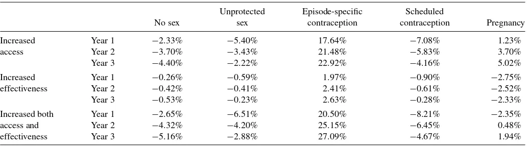
Our second policy simulation focuses on making episode-specific contraception more attractive and/or more effective at preventing pregnancy. Table 10 presents the policy simulations for the population, while Table 11 conditions on having grades that were about half B’s and C’s or worse in the eighth grade. Increasing access to episode-specific contraception increases pregnancy rates in the long run. In the short run, those who have low grades see a small drop in pregnancy rates, which are undone in the long run due to changes in sexual histories. Making condoms 10% more effective at preventing pregnancy, while leaving preferences unchanged, however, results in drops in pregnancy rates in all years. While the long-run effects are smaller than the short-run effects, there is not enough of a change in behavior to compensate for the lower pregnancy rates asso-ciated with using episode-specific contraception. Increasing the effectiveness as well as access lowers pregnancy rates in both the short and the long run for those with low grades, though by year 3, the effects are minuscule. For the population, however, a crossing is observed: first pregnancy rates fall but then, as sexual behavior adjusts, pregnancy rates rise.
Taken together, the policy simulations suggest that making contraception more attractive may lead to higher pregnancy rates, particularly in the long run. However, increasing the effi-cacy of contraceptive use (yet somehow not affecting access or preferences) is likely to result in decreases in pregnancy rates both in the short and in the long run.
6. CONCLUSION
Our estimates show large transition and fixed costs to having sex. Persistence is also observed in using birth control methods such as the pill, with smaller effects for condoms. The persis-tence in sexual activity is such that policies that affect access to contraception may have very different effects in the short run compared with those in the long run. Our results suggest that increasing access to contraception may actually increase long-run pregnancy rates even when short-long-run pregnancy rates fall. On the other hand, policies that decrease access to contracep-tion, and hence sexual activity, may lower pregnancy rates in the long run. We should also point out that the high contraceptive failure rates under “typical” use of contraceptive methods play a crucial role in the main predictions of the policy experiments. With improved contraceptive use and lower failure rates, there could be programs that increase access to contraception, with a reduction in teen pregnancies both in the short and in the long run. The primary purpose of our research is to illustrate the un-intended consequences that may result if the dynamic aspects of teen decisions regarding sexual activity are ignored. In spite of the limitations that we discuss below, we believe that our work is important in showing that policy makers should be aware of such dynamic considerations when developing contraceptive policies.
It needs to be emphasized that our focus is on teen sexual behavior and pregnancy outcomes. Hence, our conclusions are not necessarily applicable to older individuals. For example, Goldin and Katz (2002) provided evidence on the benefits of the availability of oral contraception to women of college-going and older ages. In our analysis, we also did not examine the ef-fects of access to contraception on the incidence of STDs. This is another factor that could be important in determining appro-priate policies regarding access to contraception, particularly condoms.
There are many other factors, however, that may also point toward increased access to contraception having negative con-sequences. For example, Akerlof, Yellen, and Katz (1996) ar-gued that contraception and birth control changed the bargain-ing terms between men and women, and led to an increase in out-of-wedlock births. We also did not examine the effects of peer networks or multiplicity of sexual partners on teen sex-ual decisions and pregnancy outcomes, both of which may lead to greater access to contraception having negative effects in the long run. For example, we may see fixed costs in the form of a moral or psychological barrier the first time one has sex outside of a committed relationship. To the degree that increased access to contraception encourages experimentation outside the committed relationship, habit persistence may again lead to greater access to contraception, thus increasing teen pregnancy rates. Future research that extends our analysis to incorporate factors such as STDs, bargaining in relationships, and multiplicity of partners will improve our understanding of the consequences of increased access to contraception for teens.
An alternative explanation of why there is so much persis-tence in sexual activity in the data is that the individual-level heterogeneity that we model as permanent is actually time-varying. In this case, the persistence observed in the data would not be endogenous to past behaviors but would reflect exoge-nous taste shocks that may be persistent over time. The policy implications of these two explanations are very different. Un-der the time-varying heterogeneity, only our short-run policy simulations are relevant. Our data are not rich enough to dis-tinguish between these two hypotheses. Moreover, with rare exceptions (e.g., Pakes 1987), the convention in the dynamic discrete-choice literature has been to allow for serial correla-tion between observed variables but not between unobserved variables. As in our work, this is commonly done using the procedure proposed by Heckman and Singer (1984), which al-lows for permanent unobserved heterogeneity. Furthermore, in the spirit of Stigler and Becker (1977), we have eschewed an explanation based on time-varying unobserved heterogeneity in preferences. In our context, an additional empirical argument in favor of the permanent unobserved heterogeneity approach is that most of biological maturation has already occurred by age 14 (Zabin et al.1986; Chumelea et al.2003). In making these conventional assumptions, we find strong evidence of habit per-sistence. If, as our results suggest, the persistence observed in the data is indeed behavior-driven, even if partially, then the long-run implications of our simulations need to be considered seriously in the development of policies, given the potential for unintended consequences. Finally, even if one remains skepti-cal about our point estimates of the level of habit persistence,
Table A.1. Transition parameters
Mother working Intact family Leave home
Coeff. Std. error Coeff. Std. error Coeff. Std. error
Lag mother works 3.334 0.069 −0.800 0.252 −0.123 0.112
Lag intact family −0.233 0.073 −0.859 0.116
Black 0.053 0.984 −0.597 0.267 −0.607 0.137
Age 0.009 0.027 0.050 0.085 0.617 0.049
Mother prays −0.149 0.070 0.427 0.233
Mother some college 0.320 0.084 0.140 0.262 −0.239 0.132
Mother college graduate or more 0.450 0.096 0.756 0.315 −0.586 0.176
Math score (00’s) −0.071 0.060
Constant −1.262 0.165 3.785 0.510 −5.204 0.301
Observations 6918 3822 5870
we believe that our analysis shows conditions under standard economic assumptions where contraception policy could un-dermine its own objectives.
APPENDIX
In this Appendix, we show the estimates of the transition pa-rameters as well as the papa-rameters of the terminal value function. In particular, we show results on whether or not one’s mother works full time, whether a divorce occurs, and whether the in-dividual lives with his/her biological mother. This last measure is designed to capture whether the individual no longer lives at home, without modeling every possible living arrangement. We assume that the state variables at timetdepend only on the state variables at timet−1:
q(st|st−1)=q(st|st−1, st−2, . . .).
We assume that each follows a logit process subject to the fol-lowing restrictions:
1. Divorce is an absorbing state.
2. No longer living with one’s biological mother is an absorbing state.
Since we cannot distinguish between full-time and part-time work for the mother in wave 1, we estimate the transitions using outcomes from waves 3–5, with the corresponding lagged values coming from waves 2–4.
Table A.2. Terminal value function for pregnancy
Coefficient Std. error
Black −1.6838 0.7359
Adjusted test score −2.3740 0.9564
Household income (000’s) −0.1273 0.2880
Mother some college −0.1683 0.7229
Mother college graduate or more −2.0338 0.9302
Grades in eighth grade 1.7295 0.4689
Test score squared −0.2974 0.1746
Test score times income 0.1300 0.0845
Test score times grades 0.3722 0.1503
Income squared −0.0053 0.0075
Income times grades 0.0006 0.0461
Grades squared −0.2493 0.0557
Table A.1 presents the estimates of the logit parameters, where the estimates were obtained by maximum likelihood. The most significant predictor of one’s mother working full time at timetis whether one’s mother worked full time at timet−1. Living with both biological parents reduces the probability of the mother working, though this effect is less than one-tenth the size of the lagged mother working effect. The effect of a pray-ing mother is also negative, but smaller and only marginally significant. The coefficients on age and black are small and insignificant.
The probability of the biological family remaining intact at timetfalls if the mother worked at timet−1. A mother who prayed regularly in 1997 increases the probability of the fam-ily remaining intact, while black families are significantly more likely to experience divorce. An intact family at timet−1 sig-nificantly lowers the probability an individual will leave home, as does being black and having higher test scores. Not sur-prisingly, age has a strong positive effect on the probability of leaving home.
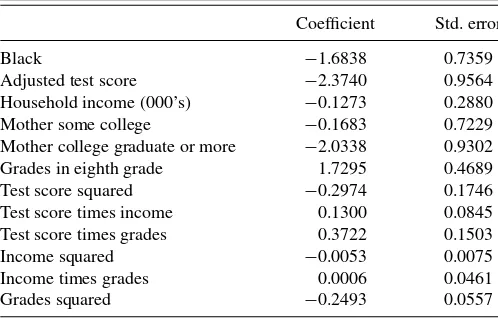
We specify the terminal value function for pregnancy flexibly in the hope of accounting for heterogeneity in labor market returns and the cost a pregnancy imposes on those labor market returns. Note that embedded in this terminal value function is the fact that individuals can abort. Absent abortion, the human capital measures would likely take on an even greater role. We approximate a terminal value function using linear terms for race, mother’s education, test scores, grades in eighth grade, and household income. We then put in squared terms and interactions for all non-dummy variables (test scores, grades, and household income). Results are reported in Table A.2.
ACKNOWLEDGMENTS
We thank Jacob Klerman, Shannon Seitz, Jim Walker, and seminar participants at Carnegie Mellon, Clemson University, the IRP Summer Research Workshop, the University of Mary-land, Northwestern University, and the winter and summer meet-ings of the Econometric Society. This research was partially funded by the National Institute for Child Health and Human Development (R03 HD042817-01A1). The views expressed are those of the authors and do not represent the opinions of the Centers for Disease Control and Prevention.
[Received June 2009. Revised November 2011.]