Hypothesis Testing Using z- and t-tests
In hypothesis testing, one attempts to answer the following question: If the null hypothesis is assumed to be true, what is the probability of obtaining the observed result, or any more extreme result that is favourable to the alternative hypothesis?1 In order to tackle this question, at least in the context of z- and t-tests, one must first understand two important concepts: 1) sampling distributions of statistics, and 2) the central limit theorem.
Sampling Distributions
Imagine drawing (with replacement) all possible samples of size n from a population, and for each sample, calculating a statistic--e.g., the sample mean. The frequency distribution of those sample means would be the sampling distribution of the mean (for samples of size n drawn from that particular population).
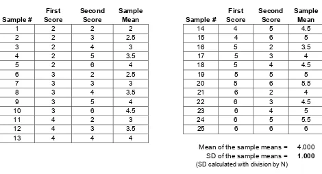
Normally, one thinks of sampling from relatively large populations. But the concept of a sampling distribution can be illustrated with a small population. Suppose, for example, that our population consisted of the following 5 scores: 2, 3, 4, 5, and 6. The population mean = 4, and the population standard deviation (dividing by N) = 1.414.
If we drew (with replacement) all possible samples of 2 from this population, we would end up with the 25 samples shown in Table 1.
Table 1: All possible samples of n=2 from a population of 5 scores.
First Second Sample First Second Sample
Sample # Score Score Mean Sample # Score Score Mean
1 2 2 2 14 4 5 4.5
2 2 3 2.5 15 4 6 5
3 2 4 3 16 5 2 3.5
4 2 5 3.5 17 5 3 4
5 2 6 4 18 5 4 4.5
6 3 2 2.5 19 5 5 5
7 3 3 3 20 5 6 5.5
8 3 4 3.5 21 6 2 4
9 3 5 4 22 6 3 4.5
10 3 6 4.5 23 6 4 5 11 4 2 3 24 6 5 5.5 12 4 3 3.5 25 6 6 6
13 4 4 4
Mean of the sample means = 4.000 SD of the sample means = 1.000
(SD calculated with division by N)
1
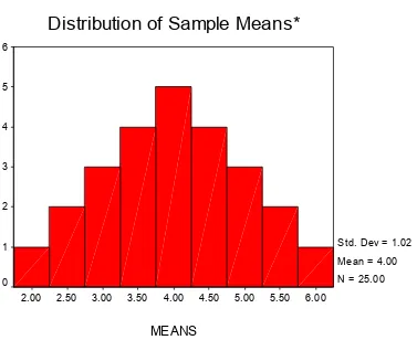
The 25 sample means from Table 1 are plotted below in Figure 1 (a histogram). This distribution of sample means is called the sampling distribution of the mean for samples of n=2 from the population of interest (i.e., our population of 5 scores).
Figure 1: Sampling distribution of the mean for samples of n=2 from a population of N=5.
I suspect the first thing you noticed about this figure is peaked in the middle, and symmetrical about the mean. This is an important characteristic of sampling distributions, and we will return to it in a moment.
You may have also noticed that the standard deviation reported in the figure legend is 1.02, whereas I reported SD = 1.000 in Table 1. Why the discrepancy? Because I used the population SD formula (with division by N) to compute SD = 1.000 in Table 1, but SPSS used the sample SD formula (with division by n-1) when computing the SD it plotted alongside the histogram. The population SD is the correct one to use in this case, because I have the entire population of 25 samples in hand.
The Central Limit Theorem (CLT)
If I were a mathematical statistician, I would now proceed to work through derivations, proving the following statements:
MEANS
6.00 5.50 5.00 4.50 4.00 3.50 3.00 2.50 2.00
Distribution of Sample Means*
* or "Sampling Distribution of the Mean" 6
5
4
3
2
1
0
1. The mean of the sampling distribution of the mean = the population mean
2. The SD of the sampling distribution of the mean = the standard error (SE) of the mean = the population standard deviation divided by the square root of the sample size
Putting these statements into symbols:
{ mean of the sample means = the population mean }
X X
µ =µ (1.1)
{ SE of mean = population SD over square root of n }
X X
n
σ
σ = (1.2)
But alas, I am not a mathematical statistician. Therefore, I will content myself with telling you that these statements are true (those of you who do not trust me, or are simply curious, may consult a mathematical stats textbook), and pointing to the example we started this chapter with. For that population of 5 scores, µ =4and σ =1.414. As shown in Table 1, µX = =µ 4, and
1.000
X
σ = . According to equation (1.2), if we divide the population SD by the square root of the sample size, we should obtain the standard error of the mean. So let's give it a try:
1.414
.9998 1
2
n
σ = = (1.3)
When I performed the calculation in Excel and did not round off σ to 3 decimals, the solution worked out to 1 exactly. In the Excel worksheet that demonstrates this, you may also change the values of the 5 population scores, and should observe that σX =σ nfor any set of 5 scores you choose. Of course, these demonstrations do not prove the CLT (see the aforementioned math-stats books if you want proof), but they should reassure you that it does indeed work.
What the CLT tells us about the shape of the sampling distribution
The central limit theorem also provides us with some very helpful information about the shape of the sampling distribution of the mean. Specifically, it tells us the conditions under which the sampling distribution of the mean is normally distributed, or at least approximately normal, where approximately means close enough to treat as normal for practical purposes.
The shape of the sampling distribution depends on two factors: the shape of the population from which you sampled, and sample size. I find it useful to think about the two extremes:
2. If the population from which you sample is extremely non-normal, the sampling distribution of the mean will still be approximately normal given a large enough sample size (e.g., some authors suggest for sample sizes of 300 or greater).
So, the general principle is that the more the population shape departs from normal, the greater the sample size must be to ensure that the sampling distribution of the mean is approximately normal. This tradeoff is illustrated in the following figure, which uses colour to represent the shape of the sampling distribution (purple = non-normal, red = normal, with the other colours representing points in between).
Does n have to be ≥ 30?
Some textbooks say that one should have a sample size of at least 30 to ensure that the sampling distribution of the mean is approximately normal. The example we started with (i.e., samples of
positive skew in the population, the distribution of sample means is near enough to normal for the normal approximation to be useful.
What is the rule of 30 about then?
In the olden days, textbook authors often did make a distinction between small-sample and large-sample versions of t-tests. The small- and large-sample versions did not differ at all in terms of how t was calculated. Rather, they differed in how/where one obtained the critical value to which they compared their computed t-value. For the small-sample test, one used the critical value of t, from a table of critical t-values. For the large-sample test, one used the critical value of z, obtained from a table of the standard normal distribution. The dividing line between small and large samples was usually n = 30 (or sometimes 20).
alpha = .05 (2-tailed) as a function of sample size. Notice that when n ≥ 30 (or even 20), the critical values of t are very close to 1.96, the critical value of z.
Nowadays, we typically use statistical software to perform t-tests, and so we get a p-value computed using the appropriate t-distribution, regardless of the sample size. Therefore the distinction between small- and large-sample t-tests is no longer relevant, and has disappeared from most modern textbooks.
The sampling distribution of the mean and z-scores
When you first encountered z-scores, you were undoubtedly using them in the context of a raw score distribution. In that case, you calculated the z-score corresponding to some value of X as follows:
X X
X X
z µ µ
σ− σ−
= = (1.4)
And, if the distribution of X was normal, or at least approximately normal, you could then take that z-score, and refer it to a table of the standard normal distribution to figure out the proportion of scores higher than X, or lower than X, etc.
X X
X X
z
n
µ µ
σ
σ− −
= = (1.5)
This is the same formula, but with X in place of X, and σX in place of σX . And, if the sampling distribution of X is normal, or at least approximately normal, we may then refer this value of z to the standard normal distribution, just as we did when we were using raw scores. (This is where the CLT comes in, because it tells the conditions under which the sampling distribution of
X is approximately normal.)
An example. Here is a (fictitious) newspaper advertisement for a program designed to increase intelligence of school children2:
As an expert on IQ, you know that in the general population of children, the mean IQ = 100, and the population SD = 15 (for the WISC, at least). You also know that IQ is (approximately) normally distributed in the population. Equipped with this information, you can now address questions such as:
If the n=25 children from Dundas are a random sample from the general population of children,
a) What is the probability of getting a sample mean of 108 or higher? b) What is the probability of getting a sample mean of 92 or lower?
c) How high would the sample mean have to be for you to say that the probability of getting a mean that high (or higher) was 0.05 (or 5%)?
d) How low would the sample mean have to be for you to say that the probability of getting a mean that low (or lower) was 0.05 (or 5%)?
2
The solutions to these questions are quite straightforward, given everything we have learned so far in this chapter. If we have sampled from the general population of children, as we are assuming, then the population from which we have sampled is at least approximately normal. Therefore, the sampling distribution of the mean will be normal, regardless of sample size. Therefore, we can compute a z-score, and refer it to the table of the standard normal distribution.
So, for part (a) above:
And from a table of the standard normal distribution (or using a computer program, as I did), we can see that the probability of a z-score greater than or equal to 2.667 = 0.0038. Translating that back to the original units, we could say that the probability of getting a sample mean of 108 (or greater) is .0038 (assuming that the 25 children are a random sample from the general
population).
For part (b), do the same, but replace 108 with 92:
92 100 8
Because the standard normal distribution is symmetrical about 0, the probability of a z-score equal to or less than -2.667 is the same as the probability of a z-score equal to or greater than 2.667. So, the probability of a sample mean less than or equal to 92 is also equal to 0.0038. Had we asked for the probability of a sample mean that is either 108 or greater, or 92 or less, the answer would be 0.0038 + 0.0038 = 0.0076.
Part (c) above amounts to the same thing as asking, "What sample mean corresponds to a z-score of 1.645?", because we know that p z( ≥1.645)=0.05. We can start out with the usual z-score formula, but need to rearrange the terms a bit, because we know that z = 1.645, and are trying to determine the corresponding value of X.
(
)
{ cross-multiply to get to next line }
z { add to both sides }
z { switch sides }
z 1.645 15 25 100 104.935
So, had we obtained a sample mean of 105, we could have concluded that the probability of a mean that high or higher was .05 (or 5%).
For part (d), because of the symmetry of the standard normal distribution about 0, we would use the same method, but substituting -1.645 for 1.645. This would yield an answer of 100 - 4.935 = 95.065. So the probability of a sample mean less than or equal to 95 is also 5%.
The single sample z-test
It is now time to translate what we have just been doing into the formal terminology of
hypothesis testing. In hypothesis testing, one has two hypotheses: The null hypothesis, and the alternative hypothesis. These two hypotheses are mutually exclusive and exhaustive. In other words, they cannot share any outcomes in common, but together must account for all possible outcomes.
In informal terms, the null hypothesis typically states something along the lines of, "there is no treatment effect", or "there is no difference between the groups".3
The alternative hypothesis typically states that there is a treatment effect, or that there is a difference between the groups. Furthermore, an alternative hypothesis may be directional or non-directional. That is, it may or may not specify the direction of the difference between the groups.
0
H and H1 are the symbols used to represent the null and alternative hypotheses respectively. (Some books may use Hafor the alternative hypothesis.) Let us consider various pairs of null and alternative hypotheses for the IQ example we have been considering.
Version 1: A directional alternative hypothesis
0 1
: 100
: 100
H H
µ µ >≤
This pair of hypotheses can be summarized as follows. If the alternative hypothesis is true, the sample of 25 children we have drawn is from a population with mean IQ greater than 100. But if the null hypothesis is true, the sample is from a population with mean IQ equal to or less than 100. Thus, we would only be in a position to reject the null hypothesis if the sample mean is greater than 100 by a sufficient amount. If the sample mean is less than 100, no matter by how much, we would not be able to reject H0.
How much greater than 100 must the sample mean be for us to be comfortable in rejecting the null hypothesis? There is no unequivocal answer to that question. But the answer that most
3
disciplines use by convention is this: The difference between X and µ must be large enough that the probability it occurred by chance (given a true null hypothesis) is 5% or less.
The observed sample mean for this example was 108. As we saw earlier, this corresponds to a z-score of 2.667, and p z( ≥2.667)=0.0038. Therefore, we could reject H0, and we would act as
if the sample was drawn from a population in which mean IQ is greater than 100.
Version 2: Another directional alternative hypothesis
0 1
: 100
: 100
H H
µ µ <≥
This pair of hypotheses would be used if we expected the Dr. Duntz's program to lower IQ, and if we were willing to include an increase in IQ (no matter how large) under the null hypothesis. Given a sample mean of 108, we could stop without calculating z, because the difference is in the wrong direction. That is, to have any hope of rejecting H0, the observed difference must be in the direction specified by H1.
Version 3: A non-directional alternative hypothesis
0 1
: 100
: 100
H H
µ µ
= ≠
In this case, the null hypothesis states that the 25 children are a random sample from a population with mean IQ = 100, and the alternative hypothesis says they are not--but it does not specify the direction of the difference from 100. In the first directional test, we needed to have X >100 by a sufficient amount, and in the second directional test, X <100 by a sufficient amount in order to reject H0. But in this case, with a non-directional alternative hypothesis, we may reject H0 if
100
X < or if X >100, provided the difference is large enough.
Because differences in either direction can lead to rejection of H0, we must consider both tails of
the standard normal distribution when calculating the p-value--i.e., the probability of the
observed outcome, or a more extreme outcome favourable to H1. For symmetrical distributions like the standard normal, this boils down to taking the p-value for a directional (or 1-tailed) test, and doubling it.
Single sample t-test (whenσ is not known)
In many real-world cases of hypothesis testing, one does not know the standard deviation of the population. In such cases, it must be estimated using the sample standard deviation. That is, s
(calculated with division by n-1) is used to estimate σ. Other than that, the calculations are as we saw for the z-test for a single sample--but the test statistic is called t, not z.
In equation (1.9), notice the subscript written by the t. It says "df = n-1". The "df" stands for
degrees of freedom. "Degrees of freedom" can be a bit tricky to grasp, but let's see if we can make it clear.
Degrees of Freedom
Suppose I tell you that I have a sample of n=4 scores, and that the first three scores are 2, 3, and 5. What is the value of the 4th score? You can't tell me, given only that n = 4. It could be anything. In other words, all of the scores, including the last one, are free to vary: df = n for a sample mean.
To calculate t, you must first calculate the sample standard deviation. The conceptual formula for the sample standard deviation is:
(
)
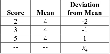
2Suppose that the last score in my sample of 4 scores is a 6. That would make the sample mean equal to (2+3+5+6)/4 = 4. As shown in Table 2, the deviation scores for the first 3 scores are -2, -1, and 1.
Table 2: Illustration of degrees of freedom for sample standard deviation
Using only the information shown in the final column of Table 2, you can deduce that x4, the 4th deviation score, is equal to -2. How so? Because by definition, the sum of the deviations about the mean = 0. This is another way of saying that the mean is the exact balancing point of the distribution. In symbols:
(
X −X)
=0∑
(1.11)So, once you have n-1 of the
(
X −X)
deviation scores, the final deviation score is determined. That is, the first n-1 deviation scores are free to vary, but the final one is not. There are n-1 degrees of freedom whenever you calculate a sample variance (or standard deviation).The sampling distribution of t
To calculate the p-value for a single sample z-test, we used the standard normal distribution. For a single sample t-test, we must use a t-distribution with n-1 degrees of freedom. As this implies, there is a whole family of t-distributions, with degrees of freedom ranging from 1 to infinity (∞ = the symbol for infinity). All t-distributions are symmetrical about 0, like the standard normal. In fact, the t-distribution with df = ∞ is identical to the standard normal distribution.
Figure 2: Probability density functions of: the standard normal distribution (the highest peak with the thinnest tails); the t-distribution with df=10 (intermediate peak and tails); and the t-distribution with df=2 (the lowest peak and thickest tails). The dotted lines are at -1.96 and +1.96, the critical values of z for a two-tailed test with alpha = .05. For all t-distributions with df < ∞, the proportion of area beyond -1.96 and +1.96 is greater than .05. The lower the degrees of freedom, the thicker the tails, and the greater the proportion of area beyond -1.96 and +1.96.
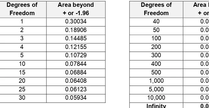
Table 3 (see below) shows yet another way to think about the relationship between the standard normal distribution and various t-distributions. It shows the area in the two tails beyond -1.96 and +1.96, the critical values of z with 2-tailed alpha = .05. With df=1, roughly 15% of the area falls in each tail of the t-distribution. As df gets larger, the tail areas get smaller and smaller, until the t-distribution converges on the standard normal when df = infinity.
Table 3: Area beyond critical values of + or -1.96 in various t-distributions. The t-distribution with df = infinity is identical to the standard normal distribution.
Degrees of Area beyond Degrees of Area beyond
Freedom + or -1.96 Freedom + or -1.96
1 0.30034 40 0.05699
2 0.18906 50 0.05558
3 0.14485 100 0.05278
4 0.12155 200 0.05138
5 0.10729 300 0.05092
10 0.07844 400 0.05069
15 0.06884 500 0.05055
20 0.06408 1,000 0.05027
25 0.06123 5,000 0.05005
30 0.05934 10,000 0.05002
Infinity 0.05000
Example of single-sample t-test.
This example is taken from Understanding Statistics in the Behavioral Sciences (3rd Ed), by Robert R. Pagano.
A researcher believes that in recent years women have been getting taller. She knows that 10 years ago the average height of young adult women living in her city was 63 inches. The standard deviation is unknown. She randomly samples eight young adult women currently residing in her city and measures their heights. The following data are obtained: [64, 66, 68, 60, 62, 65, 66, 63.]
0
The sample mean is 64.25. Because the population standard deviation is not known, we must estimate it using the sample standard deviation.
2
2 2 2
( )
sample SD
1
(64 64.25) (66 64.25) ...(63 64.25)
2.5495
We can now use the sample standard deviation to estimate the standard error of the mean:
2.5495
Estimated SE of mean = 0.901
8 conditional probability4 of obtaining a t-statistic with absolute value equal to or greater than 1.387 = 0.208. Therefore, assuming that alpha had been set at the usual .05 level, the researcher cannot reject the null hypothesis.
I performed the same test in SPSS (AnalyzeÆCompare MeansÆOne sample t-test), and obtained the same results, as shown below.
T-TEST
/TESTVAL=63 /* <-- This is where you specify the value of mu */ /MISSING=ANALYSIS
/VARIABLES=height /* <-- This is the variable you measured */ /CRITERIA=CIN (.95) .
One-Sample Test
Paired (or related samples) t-test
Another common application of the t-test occurs when you have either 2 scores for each person (e.g., before and after), or when you have matched pairs of scores (e.g., husband and wife pairs, or twin pairs). The paired t-test may be used in this case, given that its assumptions are met adequately. (More on the assumptions of the various t-tests later).
Quite simply, the paired t-test is just a single-sample t-test performed on the difference scores. That is, for each matched pair, compute a difference score. Whether you subtract 1 from 2 or vice versa does not matter, so long as you do it the same way for each pair. Then perform a single-sample t-test on those differences.
The null hypothesis for this test is that the difference scores are a random sample from a
population in which the mean difference has some value which you specify. Often, that value is zero--but it need not be.
For example, suppose you found some old research which reported that on average, husbands were 5 inches taller than their wives. If you wished to test the null hypothesis that the difference is still 5 inches today (despite the overall increase in height), your null hypothesis would state that your sample of difference scores (from husband/wife pairs) is a random sample from a population in which the mean difference = 5 inches.
In the equations for the paired t-test, X is often replaced with D, which stands for the mean difference.
Example of paired t-test
This example is from the Study Guide to Pagano’s book Understanding Statistics in The Behavioral Sciences (3rd Edition).
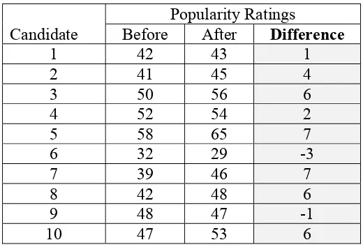
A political candidate wishes to determine if endorsing increased social spending is likely to affect her standing in the polls. She has access to data on the popularity of several other candidates who have endorsed increases spending. The data was available both before and after the candidates announced their positions on the issue [see Table 4].
Table 4: Data for paired t-test example.
Popularity Ratings
Candidate Before After Difference
1 42 43 1
2 41 45 4
3 50 56 6
4 52 54 2
5 58 65 7
6 32 29 -3
7 39 46 7
8 42 48 6
9 48 47 -1
10 47 53 6
I entered these BEFORE and AFTER scores into SPSS, and performed a paired t-test as follows:
T-TEST
PAIRS= after WITH before (PAIRED) /CRITERIA=CIN(.95)
/MISSING=ANALYSIS.
This yielded the following output.
Paired Samples Statistics
48.60 10 9.489 3.001
45.10 10 7.415 2.345
AFTER BEFORE Pair
1
Mean N Std. Deviation
Std. Error Mean
Paired Samples Correlations
10 .940 .000
AFTER & BEFORE Pair 1
Paired Samples Test
3.50 3.567 1.128 .95 6.05 3.103 9 .013
AFTER - BEFORE Pair 1
Mean Std. Deviation
Std. Error
Mean Lower Upper 95% Confidence
Interval of the Difference Paired Differences
t df Sig. (2-tailed)
The first output table gives descriptive information on the BEORE and AFTER popularity ratings, and shows that the mean is higher after politicians have endorsed increased spending.
The second output table gives the Pearson correlation (r) between the BEFORE and AFTER scores. (The correlation coefficient is measure of the direction and strength of the linear relationship between two variables. I will say more about it in a later section called Testing the significance of Pearson r.)
The final output table shows descriptive statistics for the AFTER – BEFORE difference scores, and the t-value with it’s degrees of freedom and p-value.
The null hypothesis for this test states that the mean difference in the population is zero. In other words, endorsing increased social spending has no effect on popularity ratings in the population from which we have sampled. If that is true, the probability of seeing a difference of 3.5 points or more is 0.013 (the p-value). Therefore, the politician would likely reject the null hypothesis, and would endorse increased social spending.
The same example done using a one-sample t-test
Earlier, I said that the paired t-test is really just a single-sample t-test done on difference scores. Let’s demonstrate for ourselves that this is really so. Here are the BEFORE, AFTER, and DIFF scores from my SPSS file. (I computed the DIFF scores using “compute diff = after – before.”)
BEFORE AFTER DIFF
42 43 1 41 45 4 50 56 6 52 54 2 58 65 7 32 29 -3 39 46 7 42 48 6 48 47 -1 47 53 6
Number of cases read: 10 Number of cases listed: 10
T-TEST
/TESTVAL=0
/MISSING=ANALYSIS /VARIABLES=diff
/CRITERIA=CIN (.95) .
The output is shown below.
One-Sample Statistics
10 3.50 3.567 1.128
DIFF
N Mean Std. Deviation
Std. Error Mean
One-Sample Test
3.103 9 .013 3.50 .95 6.05
DIFF
t df Sig. (2-tailed)
Mean
Difference Lower Upper 95% Confidence
Interval of the Difference Test Value = 0
Notice that the descriptive statistics shown in this output are identical to those shown for the paired differences in the first analysis. The t-value, df, and p-value are identical too, as expected.
A paired t-test for which H specifies a non-zero difference 0
The following example is from an SPSS syntax file I wrote to demonstrate a variety of t-tests.
* A researcher knows that in 1960, Canadian husbands were 5" taller * than their wives on average. Overall mean height has increased * since then, but it is not known if the husband/wife difference * has changed, or is still 5". The SD for the 1960 data is * not known. The researcher randomly selects 25 couples and * records the heights of the husbands and wives. Test the null * hypothesis that the mean difference is still 5 inches.
* H0: Mean difference in height (in population) = 5 inches. * H1: Mean difference in height does not equal 5 inches.
list all.
COUPLE HUSBAND WIFE DIFF
8.00 78.79 63.50 15.29
* We cannot use the "paired t-test procedure, because it does not * allow for non-zero mean difference under the null hypothesis. * Instead, we need to use the single-sample t-test on the difference * scores, and specify a mean difference of 5 inches under the null.
T-TEST
/TESTVAL=5 /* H0: Mean difference = 5 inches (as in past) */ /MISSING=ANALYSIS
/VARIABLES=diff /* perform analysis on the difference scores */ /CRITERIA=CIN (.95) .
.716 24 .481 .9372 -1.7654 3.6398 DIFF
* The observed mean difference = 5.9 inches.
* The null hypothesis cannot be rejected (p = 0.481).
* the mean difference = 5 inches.
* Suppose we had found that the difference in height between * husbands and wives really had decreased dramatically. In * that case, we might have found a mean difference close to 0, * which might have allowed us to reject H0. An example of * this scenario follows below.
COUPLE HUSBAND WIFE DIFF
1.00 68.78 75.34 -6.56 2.00 66.09 67.57 -1.48 3.00 71.99 69.16 2.83 4.00 74.51 69.17 5.34 5.00 67.31 68.11 -.80 6.00 64.05 68.62 -4.57 7.00 66.77 70.31 -3.54 8.00 75.33 72.92 2.41 9.00 74.11 73.10 1.01 10.00 75.71 62.66 13.05 11.00 69.01 76.83 -7.82 12.00 67.86 63.23 4.63 13.00 66.61 72.01 -5.40 14.00 68.64 76.10 -7.46 15.00 78.74 68.53 10.21 16.00 71.66 62.65 9.01 17.00 73.43 70.46 2.97 18.00 70.39 79.99 -9.60 19.00 70.15 64.27 5.88 20.00 71.53 69.07 2.46 21.00 57.49 81.21 -23.72 22.00 68.95 69.92 -.97 23.00 77.60 70.70 6.90 24.00 72.36 67.79 4.57 25.00 72.70 67.50 5.20
Number of cases read: 25 Number of cases listed: 25
T-TEST
/TESTVAL=5 /* H0: Mean difference = 5 inches (as in past) */ /MISSING=ANALYSIS
/VARIABLES=diff /* perform analysis on the difference scores */ /CRITERIA=CIN (.95) .
T-Test
One-Sample Statistics
25 .1820 7.76116 1.55223
DIFF
N Mean Std. Deviation
One-Sample Test
-3.104 24 .005 -4.8180 -8.0216 -1.6144
DIFF
* The mean difference is about 0.2 inches (very close to 0). * Yet, because H0 stated that the mean difference = 5, we * are able to reject H0 (p = 0.005).
Unpaired (or independent samples) t-test
Another common form of the t-test may be used if you have 2 independent samples (or groups). The formula for this version of the test is given in equation (1.17).
(independent) samples, or the difference between group means. The right side of the numerator,
1 2
As indicated above, the null hypothesis for this test specifies a value for (µ µ1− 2), the difference specify a non-zero difference between the population means. Second, it reminds me that all t-tests have a common format, which I will describe in a section to follow.
The unpaired (or independent samples) t-test has df = + −n1 n2 2. As discussed under the
Single-sample t-test, one degree of freedom is lost whenever you calculate a sum of squares (SS). To perform an unpaired t-test, we must first calculate both SS1and SS2, so two degrees of
freedom are lost.
Example of unpaired t-test
The following example is from Understanding Statistics in the Behavioral Sciences (3rd Ed), by Robert R. Pagano.
I entered these scores in SPSS as follows:
To run an unpaired t-test: AnalyzeÆCompare MeansÆIndependent Samples t-test. The syntax and output follow.
.001 .972 3.998 15 .001 6.26 1.565 2.922 9.593
3.995 13.028 .002 6.26 1.566 2.874 9.640
The null hypothesis for this example is that the 2 groups of children are 2 random samples from populations with the same mean levels of lead concentration in the blood. The p-value is 0.001, which is less than the 0.01 specified in the question. So we would reject the null hypothesis. Putting it another way, we would act as if living close to the smelter is causing an increase in lead concentration in the blood.
Testing the significance of Pearson r
Pearson r refers to the Pearson Product-Moment Correlation Coefficient. If you have not learned about it yet, it will suffice to say for now that r is a measure of the strength and direction of the linear (i.e., straight line) relationship between two variables X and Y. It can range in value from -1 to +1.
Negative values indicate that there is a negative (or inverse) relationship between X and Y: i.e., as X increases, Y decreases. Positive values indicate that there is a positive relationship: as X increases, Y increases.
If r=0, there is no linear relationship between X and Y. If r = -1 or +1, there is a perfect linear relationship between X and Y: That is, all points fall exactly on a straight line. The further r is from 0, the better the linear relationship.
Pearson r is calculated using matched pairs of scores. For example, you might calculate the correlation between students' scores in two different classes. Often, these pairs of scores are a sample from some population of interest. In that case, you may wish to make an inference about the correlation in the population from which you have sampled.
The Greek letter rho is used to represent the correlation in the population. It looks like this: ρ. As you may have already guessed, the null hypothesis specifies a value for ρ. Often that value is 0. In other words, the null hypothesis often states that there is no linear relationship between X and Y in the population from which we have sampled. In symbols:
0
You may recall the following output from the first example of a paired t-test (with BEFORE and
The number in the “Correlation” column is a Pearson r. It indicates that there is a very strong and positive linear relationship between BEFORE and AFTER scores for the 10 politicians. The p-value (Sig.) is for a t-test of the null hypothesis that there is no linear relationship between BEFORE and AFTER scores in the population of politicians from which the sample was drawn. The p-value indicates the probability of observing a correlation of 0.94 or greater (or –0.94 or less, because it’s two-tailed) if the null hypothesis is true.
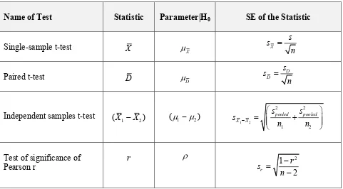
General format for all z- and t-tests
You may have noticed that all of the z- and t-tests we have looked at have a common format. The formula always has 3 components, as shown below:
0
The numerator always has some statistic (e.g., a sample mean, or the difference between two independent sample means) minus the value of the corresponding parameter, given that H0 is true. The denominator is the standard error of the statistic in the numerator. If the population standard deviation is known (and used to calculate the standard error), the test statistic is z. if the population standard deviation is not known, it must be estimated with the sample standard
deviation, and the test statistic is t with some number of degrees of freedom. Table 5 lists the 3 components of the formula for the t-tests we have considered in this chapter. For all of these tests but the first, the null hypothesis most often specifies that the value of the parameter is equal to zero. But there may be exceptions.
Similarity of standard errors for single-sample and unpaired t-tests
People often fail to see any connection between the formula for the standard error of the mean, and the standard error of the difference between two independent means. Nevertheless, the two formulae are very similar, as shown below.
Table 5: The 3 components of the t-formula for t-tests described in this chapter.
Name of Test Statistic Parameter|H0 SE of the Statistic
Single-sample t-test X µX X key requirement (or assumption) for any t-test is that the statistic in the numerator must have a sampling distribution that is normal. This will be the case if the populations from which you have sampled are normal. If the populations are not normal, the sampling distribution may still be approximately normal, provided the sample sizes are large enough. (See the discussion of the Central Limit Theorem earlier in this chapter.) The assumptions for the individual t-tests we have considered are given in Table 6.
A little more about assumptions for t-tests
Many introductory statistics textbooks list the following key assumptions for t-tests:
1. The data must be sampled from a normally distributed population (or populations in case of a two-sample test).
2. For two-sample tests, the two populations must have equal variances.
3. Each score (or difference score for the paired t-test) must be independent of all other scores.
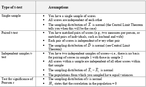
Table 6: Assumptions of various t-tests.
Type of t-test Assumptions
Single-sample • You have a single sample of scores
• All scores are independent of each other
• The sampling distribution of X is normal (the Central Limit Theorem tells you when this will be the case)
Paired t-test • You have matched pairs of scores (e.g., two measures per person, or matched pairs of individuals, such as husband and wife)
• Each pair of scores is independent of every other pair
• The sampling distribution of D is normal (see Central Limit Theorem)
Independent samples
t-test •
You have two independent samples of scores—i.e., there is no basis for pairing of scores in sample 1 with those in sample 2
• All scores within a sample are independent of all other scores within that sample
• The sampling distribution of X1−X2 is normal
• The populations from which you sampled have equal variances Test for significance of
Pearson r •
The sampling distribution of r is normal
• H0 states that the correlation in the population = 0
Let’s stop and think about this for a moment in the context of an unpaired t-test. A normal distribution ranges from minus infinity to positive infinity. So in truth, none of us who are dealing with real data ever sample from normally distributed populations. Likewise, it is a virtual impossibility for two populations (at least of the sort that would interest us as researchers) to have exactly equal variances. The upshot is that we never really meet the assumptions of normality and homogeneity of variance.
Therefore, what the textbooks ought to say is that if one was able to sample from two normally distributed populations with exactly equal variances (and with each score being independent of all others), then the unpaired t-test would be an exact test. That is, the sampling distribution of t
under a true null hypothesis would be given exactly by the t-distribution with df = n1 + n2 – 2. Because we can never truly meet the assumptions of normality and homogeneity of variance, t -tests on real data are approximate -tests. In other words, the sampling distribution of t under a true null hypothesis is approximated by the t-distribution with df = n1 + n2 – 2.
So, rather than getting ourselves worked into a lather over normality and homogeneity of variance (which we know are not true), we ought to instead concern ourselves with the
conditions under which the approximation is good enough to use (much like we do when using other approximate tests, such as Pearson’s chi-square).
The t-test approximation will be poor if the populations from which you have sampled are too far from normal. But how far is too far? Some folks use statistical tests of normality to address this issue (e.g., Kolmogorov-Smirnov test; Shapiro-Wilks test). However, statistical tests of
normality are ill advised. Why? Because the seriousness of departure from normality is
inversely related to sample size. That is, departure from normality is most grievous when sample sizes are small, and becomes less serious as sample sizes increase.6 Tests of normality have very little power to detect departure from normality when sample sizes are small, and have too much power when sample sizes are large. So they are really quite useless.
A far better way to “test” the shape of the distribution is to ask yourself the following simple question:
Is it fair and honest to describe the two distributions using means and SDs?
If the answer is YES, then it is probably fine to proceed with your t-test. If the answer is NO (e.g., due to severe skewness, or due to the scale being too far from interval), then you should consider using another test, or perhaps transforming the data. Note that the answer may be YES even if the distributions are somewhat skewed, provided they are both skewed in the same direction (and to the same degree).
The second guideline, concerning homogeneity of variance, is that if the larger of the two variances is no more than 4 times the smaller,7 the t-test approximation is probably good enough—especially if the sample sizes are equal. But as Howell (1997, p. 321) points out,
It is important to note, however, that heterogeneity of variance and unequal sample sizes do not mix. If you have reason to anticipate unequal variances, make every effort to keep your sample sizes as equal as possible.
Note that if the heterogeneity of variance is too severe, there are versions of the independent groups t-test that allow for unequal variances. The method used in SPSS, for example, is called the Welch-Satterthwaite method. See the appendix for details.
All models are wrong
Finally, let me remind you of a statement that is attributed to George Box, author of a well-known book on design and analysis of experiments:
All models are wrong. Some are useful.
This is a very important point—and as one of my colleagues remarked, a very liberating
statement. When we perform statistical analyses, we create models for the data. By their nature, models are simplifications we use to aid our understanding of complex phenomena that cannot be grasped directly. And we know that models are simplifications (e.g., I don’t think any of the early atomic physicists believed that the atom was actually a plum pudding.) So we should not find it terribly distressing that many statistical models (e.g., t-tests, ANOVA, and all of the other
6
As sample sizes increase, the sampling distribution of the mean approaches a normal distribution regardless of the shape of the original population. (Read about the central limit theorem for details.)
7
parametric tests) are approximations. Despite being wrong in the strictest sense of the word, they can still be very useful.
References
Howell, D.C. (1997). Statistics for psychology (4th Ed). Belmont, CA: Duxbury.
Appendix: The
Unequal Variances
t
-test in SPSS
Denominator for the independent groups t-test, equal variances assumed
2 2
Denominator for independent t-test, unequal variances assumed
2 2
• Suppose the two sample sizes are quite different
• If you use the equal variance version of the test, the larger sample contributes more to the pooled variance estimate (see first line of equation A-1)
• But if you use the unequal variance version, both samples contribute equally to the pooled variance estimate
Sampling distribution of t
• For the equal variance version of the test, the sampling distribution of the t-value you calculate (under a true null hypothesis) is the t-distribution with df = n1 + n2 – 2
• For the unequal variance version, there is some dispute among statisticians about what is the appropriate sampling distribution of t
• There have been a few attempts to define exactly how much less.
• Some books (e.g., Biostatistics: The Bare Essentials describe a method that involves use of the harmonic mean.
• SPSS uses the Welch-Satterthwaite solution. It calcuates the adjusted df as follows:
2
2 2
1 2
1 2
2 2
2 2
1 2
1 2
1
1
21
s
s
n
n
df
s
s
n
n
n
n
+
=
+
−
−
(A-3)