Planarizable Supersymmetric Quantum Toboggans
⋆Miloslav ZNOJIL
Nuclear Physics Institute ASCR, 250 68 ˇReˇz, Czech Republic E-mail: [email protected]
URL: http://gemma.ujf.cas.cz/~znojil/
Received November 30, 2010, in final form February 21, 2011; Published online February 25, 2011
doi:10.3842/SIGMA.2011.018
Abstract. In supersymmetric quantum mechanics the emergence of a singularity may lead to the breakdown of isospectrality between partner potentials. One of the regularization recipes is based on a topologically nontrivial, multisheeted complex deformations of the line of coordinatexgiving the so called quantum toboggan models (QTM). The consistent theoretical background of this recipe is briefly reviewed. Then, certain supersymmetric QTM pairs are shown exceptional and reducible to doublets of non-singular ordinary differential equations a.k.a. Sturm–Schr¨odinger equations containing a weighted energyE → EW(x) and living insinglecomplex plane.
Key words: supersymmetry; Schr¨odinger equation; complexified coordinates; changes of
variables; single-complex-plane images of Riemann surfaces
2010 Mathematics Subject Classification: 81Q60; 81Q12; 46C15; 81Q10; 34L20; 47A75;
47B50
1
Introduction
Within the framework of the standard supersymmetric quantum mechanics (SUSY QM as re-viewed, e.g., by Cooper et al. [1]) the interaction potentials V(x) must be assumed regular. Otherwise, in a way pointed out by Jevicki and Rodrigues [2] the usual correspondence between spectra of the SUSY-related “partner” Hamiltonians might disappear. The SUSY-induced pa-rallels between the bound states generated by the partner potentials would break down [3]. The main phenomenological merit of the formalism would be lost. In the language of mathematics, with the singularity emerging at least in one of the partner potentials, even the respective Hilbert spaces may become different. For illustration of details one may consult, e.g., Fig. 12.1 of [1] or the explicit construction of an example by Das and Pernice [4].
In the spirit of the PT-symmetric quantum mechanics (PTS QM, introduced and made popular mainly in [5, 6, 7, 8, 9, 10]) we returned to the Jevicki’s and Rodrigues’ problem. In a comment [11] on [4] we recommended the regularization of the strong singularities inV(x) me-diated by a suitablesmallcomplex deformation of the line of coordinates. The requirement of the smallness of thePT-symmetric deformationC →Rof the line of coordinates appeared essential as long as the regularized Hamiltonians themselves became manifestly non-Hermitian,H6=H†. During the subsequent development of the theory a full understanding has been achieved of the formal foundations of the recipe based on the use of non-Hermitian operators of observables with real spectra. The recent reviews [12, 13, 14, 15] my be recalled as confirming the full compatibility of PT-symmetric models with the standard postulates of quantum mechanics.
The resulting extension of the practical scope of quantum theory opened the path towards the proposal of a new class of regularization recipes [16,17]. They may be characterized by the
⋆This paper is a contribution to the Proceedings of the Workshop “Supersymmetric Quantum
Me-chanics and Spectral Design” (July 18–30, 2010, Benasque, Spain). The full collection is available at
use of arbitrarily deformed and even topologically nontrivial complex curves x= x(s) ∈ C ⊂ C of generalized coordinates defined over certain topologically nontrivial Riemann surfaces R.
In a number of concrete non-SUSY examples [18], the latter curves Cwere, typically, chosen as spiralling around the branch points of the wave functionsψ(x). For this reason we coined the name of “quantum toboggan models” (QTM) for all of the models supported by a topologically nontrivial (i.e., multisheeted) integration curve C along which the latter wave functions ψ(x) are, by construction, analytic.
In our most recent paper on the QTM [19] we returned to [11] and indicated that the menu of possible QTM regularizations of SUSY may be broader than expected. New and surprising connections between algebraic (SUSY) and analytic properties of wave functions were recently revealed [20]. In this context the use of the regularizations leads again to a number of new open questions (cf., e.g., [21]). For this reason we are also returning to the subject in our present paper. In addition to an overall outline of the relevant parts of the theory, we plan to present here also a few new and unpublished results. First, in Section 2a compact summary will be given of the traditional role of SUSY in quantum mechanics. Second, Section 3 will review briefly the introduction and a few relevant results obtained during the most recent QTM constructions. Next, Sections 4 and 5 will offer a thorough explanation of compatibility between QTM con-structions and the standard probabilistic interpretation and postulates of quantum mechanics. The key ingredients in these explanations will be the simplification of the QTM mathematics via a “rectification” change of variables and the subsequent construction of the “standard” Hilbert space H(S) by means of the introduction of certain not entirely standard inner products.
A few open problems will finally be addressed in Section6(including also our main illustrative example of planarization) and in a few appendices. Thus, in AppendixA we shall explain that the non-Hermiticity property H 6=H† of the regularized Hamiltonians (say, of [11]) is just an artifact of an inadequate choice of the “false” Hilbert spaceH(F)where the superscript may also hint that this space is only “too friendly” (cf. also [15] for additional details). In subsequent AppendixBwe shall make use of this theoretical background attaching three Hilbert spaces to the single quantum system. In AppendixCwe shall describe a more concrete implementation of the resulting innovative “three-Hilbert-space” quantum mechanics (THS QM) to the tobogganic version of popular V(x) = ix3. Finally, all these preliminary considerations will be fructified after return to Section 6where a synthesis of the idea of SUSY with the idea of PT-symmetry will be presented (and summarized in Section7).
2
Supersymmetric Schr¨
odinger equations
Let us recall that, paradoxically, the recent intensive development of the mathematics of SUSY QM failed to reach its original goals (in particle physics) but still may be considered very successful, especially in its role of a tool for study of mutual relations between different potentials in the quantum bound state problem.
The basic idea of SYSY QM is virtually elementary: in terms of the two differential operators
A=− d
dx+W(x), B = d
dx+W(x) (1)
defined in terms of the calligraphic-font “superpotential”W(x) one constructs the calligraphic-font partitioned Hamiltonian
H=
H(U) 0 0 H(L)
=
BA 0
0 AB
, (2)
supercharges,
These operators are easily shown to generate one of the simplest SUSY algebras (cf. [1] for all the details and multiple consequences).
In the spirit of our comment [11] it is important to consider operators (1) without any additional assumption requiring the reality and regularity of the superpotentials W(x). As a consequence, operators A and B need not necessarily play the role of the usual annihilation and creation operators, etc. For the first time we used this innovative flexibility of superpoten-tials W(x) in [22] (cf. also [23]) where we managed to regularize
The choice of the new auxiliary involution operator T remained unrestricted by the algebraic considerations.
In the above-mentioned amendment of the formalism [19] we merely relaxed the involutivity property T2 =I and postulated
A=−T d
dx+T W(x), B = d dxT
−1+W(x)T−1. (4)
Now we intend to develop this idea further on.
The first technical ingredient needed for a consistent build up of the SUSY version of the theory lies in the necessary clarification of the change of the role of the Hermitian conjugation operation during and after the supersymmetrization. The discussion of this point will be given below. Here, in introduction, we would only like to remind the readers that the use of thecomplex superpotentials W =−ψ′
0/ψ0 proved extremely productive, especially by leading to many new solvable Schr¨odinger equations (cf. [24, 25]) in which the authors managed to circumvent the obstructions connected with the “seed” wave functionsψ0 having nodal zeros.
3
Tobogganic Schr¨
odinger equations
Even the earliest papers on the models described by equation (8) of Appendix A [26] already reported the emergence of the real bound-state energies for certain non-real potentials V(x) and/or for certain non-real paths of integration C(s) 6= R of the Schr¨odinger equation. These papers found their motivation in perturbation theory and their authors did not pretend to offer any truly physical predictions. The situation has changed after the publication of the influential letter [6]. The subsequent massive return of interest to the apparently non-Hermitian models with real spectra resulted in the discoveries of many new exactly solvable analytic models [27], square-well-shaped models [28], point interaction models [29], Calogero-type many-body mo-dels [30] and, last but not least, of the tobogganic models in which the paths C(s) were chosen as spiralling around the branch points of their (by assumption, analytic) wave functions ψ(x).
Teaching by example let us recall here the most elementary (viz., force-free, radial, purely kinematical) HamiltonianH of [31],
H =− d 2
dx2 +
ℓ(ℓ+ 1)
first first third third
fifth fifth
0
0
Re_x Im_x
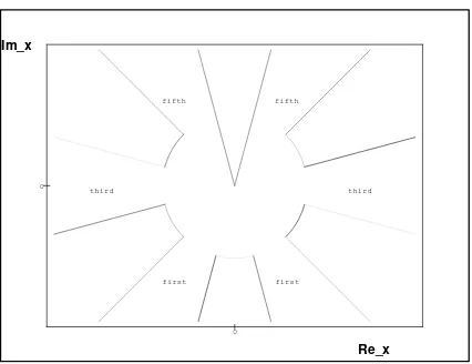
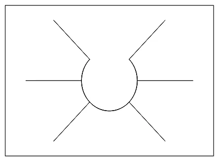
Figure 1. The allowed wedges for the non-tobogganic, single-complex-plane integration contours for potentialV(x) =x2(ix)8 and for the preselected wave-function asymptoticsψ(x)∼exp−x6/6.
In a small complex vicinity of the origin any related wave functionψ(x) has, obviously, the well known form
ψ(x) =c+ψ(+)(x) +c−ψ(−)(x),
where
ψ(+)(x) =xℓ+1+ corrections, ψ(−)(x) =x−ℓ+ corrections, |x| ≪1.
This means that at a generic real ℓ > −1/2 the corresponding Riemann surface R will posses a branch point atx= 0. Whenever this value ofℓbecomes rational, the corresponding Riemann surfaceRwill be glued of a finite number of separate sheets. Obviously, the study of the analytic properties of wave functions only becomes sufficiently well known at the integer values ofℓ(cf. also a comment on this point in [31]).
3.1 The single-Riemann-sheet (i.e., cut-plane) models
The most natural way out of the difficulties which characterize the general choice of ℓ lies, obviously, in the simplest special choice of ℓ = 0. Even then, the study of the most popular complex potentials V(q) = (iq)δq2 requires a number of technical simplifications which lead, according to the recommendations in [6], to the most stable results when the pathC(s) remains confined to a single cut complex plane. At any δ ≥ 0 one can then define an “optimal” set of curves (i.e., δ-dependent asymptotic boundary conditions) for which all of the bound-state energy levelsEnbehave as smooth functions of the couplingsλor of the other variable parameters collected in a suitable multiindex~λ entering the energies as their argument,En=En(~λ).
For illustration we may pick up, say, the asymptotically decadic potential V(x) = λ(ix)8x2 and declare, say, the specific asymptotics ψ(x) ∼ exp (−x6/6) of wave functions physical at
|x| ≫1. Then, the coupling-independent triplet of the allowed left-right-symmetric asymptotical wedges exists in a way hinted by Fig. 1 where we did setλ= 1 without loss of generality.
Naturally, beyond the single complex plane (with an upwards-oriented cut) the heuristically extremely successful left-right symmetry of curves C(s) might be also preserved – this was the basic idea of the introduction of quantum toboggans in [17].
3.2 The more-Riemann-sheets models (quantum toboggans)
0
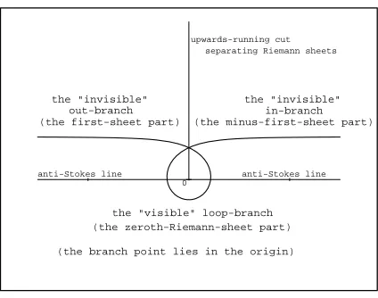
anti-Stokes line anti-Stokes line upwards-running cut
separating Riemann sheets
the "visible" loop-branch (the zeroth-Riemann-sheet part)
(the minus-first-sheet part) in-branch the "invisible"
(the first-sheet part) out-branch the "invisible"
(the branch point lies in the origin)
Figure 2. An example of a single-branch tobogganic curveC(π).
the Riemann surface R which are left-right symmetric in projection to the cut complex plane. Moreover, we shall assume that these curves remain
1) locally linear and parallelling the real axis at |s| ≪1; this means that they may be then prescribed by the formula C(α)(s) =−iε+s+O(s2) at a suitable shift-parameterε >0;
2) turning upwards by the angle α >0 during the growth of s∈ (0,∞) while disappearing “behind the cut” (i.e., to the first Riemann sheet, etc.), provided only thatα > π/2; 3) turning upwards by the angle α > 0 during the growth of t = −s∈ (0,∞) while
disap-pearing “behind the cut” (i.e., to the minus-first Riemann sheet, etc.), provided only that α > π/2;
4) encircling the branch point by the total angle 2αand becoming again approximately linear at large|s| ≫1 (cf. the illustrative sample of C(α) withα=π given in Fig.2).
At the present stage of development of the general theory of quantum toboggans [32] our in-sight in their structure based on the existing purely numerical studies of their spectra cannot still be considered satisfactory. In particular, the bad news were communicated by Gerd Wessels [33] who merely managed to show how the standard numerical methods of Runge–Kutta class suc-ceed in some of the most standard non-tobogganic models (8). His numerical algorithms failed to converge in the domains of the expected reality of the tobogganic spectra. Similar incomplete preliminary calculations were also reported by Hynek B´ıla [34].
Fortunately, our recent attempted application of perturbation theory (briefly summarized in Appendix C below) succeeded in the quantitative estimate of the topology-dependence of the tobogganic stable-bound-state spectra in the large-ℓ dynamical regime. The calculations have already been performed for the most important special case of the well known toy model where V(x)∼ix3. The current 1/ℓexpansion technique proved applicable and consistent. Our calculations led to the prediction of the nontrivial leading-order topology-dependence of the low-lying energy levels.
3.3 A quantum-toboggan example which is exactly solvable
Theorem 1 (cf. [31]). The tobogganic Schr¨odinger equation
− d
which is perturbed by the short-range potential V(r) =γ/r2 of a quantized strength
γ =
possesses a closed-form bound-state solution ψ(r) ∈ L2(C(α)) at any integer spatial dimension parameter D, integer angular momentum parameter n, integer winding number N =α/π and an “allowed” integer M = 1,2,3, . . ., M 6= 2N,4N,6N, . . ..
As long as equation (5) is solvable in terms of Bessel functions,
ψ(r) =c1√rHν(1)(κr) +c2√rHν(2)(κr), ν =ℓ+ 1/2
we have to study their asymptotics in the asymptotic (i.e., ̺≫1) wedges
• S0 ={r =−i̺eiϕ|ϕ∈(−π/2, π/2)},
• S±k={r=−ie±ikπ̺eiϕ|ϕ∈(−π/2, π/2)},k≥1.
By construction, the tobogganic contour C(α) then connects the Stokes’ wedge S0 with the Stokes’ wedge Sm where m = 2N. Thus, we are entitled to use the well known asymptotic formulae
and conclude that in S2k we may eliminate the unphysical (i.e., asymptotically non-vanishing) component Hν(1)(z) and get the physical normalizable wave function proportional to Hν(2)(z). In S2k+1, on the contrary, we encounter the physical Hν(1)(z) and unphysical Hν(2)(z). In this way we may start at s=−∞from
ψ(left)(r) =c√rHν(2)(κr) (withr ∈ S0)
and end up with ψ(right)(r) given in closed form
Hν(2) zeimπ
Obviously, the latter function will vanish at s= +∞ for the quantized angular momentaν:
mν = integer, ν 6= integer =⇒ ℓ= M −N
2N .
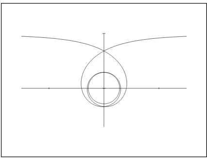
Figure 3. A tobogganic curve which three times encircles the branchpoint.
4
The Sturm–Schr¨
odinger “canonical” form of the toboggans
Once we defined quantum toboggans as ordinary differential Schr¨odinger equations integrated over paths C(s) connecting several Riemann sheets of the wave functions ψ(x), it is natural to complement, in the next step of the analysis, the single-loop tobogganic-curve of Fig. 2 by its multiply-spiralling descendants sampled, say, in Fig. 3. At the same time, in our present paper we shall not move to the next step of generalization in which more branch points are admitted inR (in this respect, e.g., [36] may be consulted).
For all of the left-right symmetric central spirals one can consider the tobogganic ordinary differential QTM Schr¨odinger equation
H(1)ψn(1)(r) =Enψn(1)(r), H(1) =− d2 dr2 +V
(1)(r)
and introduce a change of variables (say, r → y) which is, up to some constants, such that r ∼yαwith a sufficiently large exponentα∈(1,∞). Under such a mapping the two radial rays in the initial, tobogganic complexr-plane will be mapped on the two radial rays in the complex y-plane with a smaller angle between them. Thus, any angle between the radial rays becomes diminished by the mapping even when the initial rays are located on a multisheeted Riemann surface R of variable r. In this manner some of the rays which were originally hidden behind the cut (i.e., which belonged to the invisible Riemann sheets in variable r) will eventually move to the zeroth Riemann sheet in the new coordinate y, i.e., they become visible in the standard complex plane of y, say, with an upwards-running cut.
The detailed description of this technique which will rectify (i.e., straighten up) the QTM curves sampled in Figs. 2 and 3 (i.e., lower the total angle between their asymptotics) may be found elsewhere [32]. Here, let us only mention that in the literature one quite often finds the alternative, de-rectifying complex mappings x ∼ yβ with a small exponent β ∈(0,1). On Riemann surfaces this mapping acts in the opposite direction. Most often, it is used just to transform the exactly solvable harmonic oscillator into the exactly solvable bound-state part of the Coulombic (or Kepler) quantum system [37]. In the latter setting, both the initial and final coordinates remain real. The resulting, new Schr¨odinger equation for bound states acquires the form of the Sturmian eigenvalue problems where the energy appears multiplied by a non-constant (and, in our present paper, non-calligraphic-font) weight function W(y),
H(2)ψ(2)n (y) =EnW(y)ψ(2)n (y), H(2)=− d 2
In our present QTM setting we shall useα >1 and emphasize that both the initialr and finaly are complex in general. This means that in the respective usual and friendly or “false” Hilbert spacesH(F(1,2)) =L2(C) we have to deal with the manifestly non-self-adjoint operators,
W 6= [W]† and H(1,2)6=
H(1,2)†
in H(F)=H(F)(1,2). (6)
Just for illustration it is easy to verify that the change of variables
ix= (iz)2, ψn(x) =√zϕn(z)
with α = 2 returns us from the first nontrivial tobogganic form of the standard harmonic-oscillator Schr¨odinger equation to anon-tobogganicsextic-oscillator Sturm–Schr¨odinger equation Hϕ = EW ϕ which remains manifestly PT-symmetric and defined on an U-shaped contour where W >0 [38],
− d
2
dz2 + 4z
6+4α2−1/4 z2
ϕn(z) =−4Enz2ϕn(z).
In general cases the rectification strategy is often further simplified and reduced just to the use of the winding-numbered paths of both the r- or y-implementations
C(N)(s) =−i [i(s−iε)]2N+1, s∈(−∞,∞)
with integer N. More details concerning the concrete realizations of this technique should be sought elsewhere (e.g., in our review paper [32]).
5
Towards the non-Dirac metrics Θ
6
=
I
in the physical Hilbert spaces of states
5.1 The non-Sturmian constructions with W = I
The very brief account of the quantum theory using the non-standard (often called non-Di-rac [13]) assumption (6) may be found in [15] or, in an even more compressed form, in AppendixA below. Its historical roots are in fact very recent since the explicit quantum-theoretical inter-pretation ofPT-symmetric models as independently revealed by several groups of authors only dates back to the years 2001 and 2002 [7,8,9].
It is necessary to add that the basic idea of the unphysical nature of the “friendly but false” Hilbert spaces H(F) (with the trivial, often called Dirac’s metric Θ(F) =I) and of the unitary equivalence between the alternative physical realizations H(S) (with Θ(S) = Θ 6=I) and H(P) (with unfriendly Hamiltonianshbut still trivial Θ(P) =I) of the space of states already appeared in nuclear physics before 1992 [39].
Another marginal addendum to Appendix A concerns notation: one has to recollect that the physical Hilbert spaceH(S) is defined as equipped with an amended Hermitian-conjugation operation (9) which co-applies also to the operators in the form
A → A‡:= Θ−1A†Θ
such that we may deduce the reality of the spectrum ofH by its (crypto-)Hermiticity H =H‡ realized as “hidden” in space H(S). Usually one proceeds in an opposite direction. Keeping in mind the definition of the conjugation A‡ the main problem usually lies in the necessary construction of the metric operator Θ = Θ†> I.
5.2 The transition to W 6= I
There exist a few not too essential though still nontrivial differences between the non-tobogganic and tobogganic quantum systems. They may formally be reduced to the differences between the Sch¨odinger and Sturm–Schr¨odinger time-independent equations whereW =I and W 6=I, respectively.
We now have to clarify the possibility and methods of construction of the metrics Θ for toboggans, say, in their rectified Sturm–Schr¨odinger representation. This representation might also be called “planarized” (i.e., defined in a single complex plane, admissibly with cuts), but we shall rather reserve the latter term for the narrower families of the models in which all the Riemann surface R is mapped on the single complex plane with a single cut or, alternatively, without any cuts at all.
Naturally, the latter specification of the concept of the “planarizability” would be much narrower, requiring that there is just a finite number of sheets forming the planarizable Riemann surface R in question. Even in such a form its use may still prove overcomplicated from the purely pragmatic point of view. For this reason, in what follows, we shall unify and further reduce the two alternatives and speak about the planarization-mapping correspondenceR ↔C if and only if the mapping itself is given or known in an explicit form of some well-defined change of the variables.
The importance of distinguishing between the planarizable and non-planarizable QTM has not yet been addressed in the literature. This motivated also our present considerations in which we intend to emphasize that the concept of the planarizable Riemann surfaces is in fact not too robust (a small change of interaction may make them non-planarizable). At the same time, the corresponding expected enhanced sensitivity of the QTM spectra, say, to the small variations of the angular momenta ℓis not too surprising. Indeed, the similar strong-sensitivity phenomenon has already been observed even in non-tobogganic models where it was quantitatively described, e.g., by Dorey et al. [35]. Unfortunately, its quantitative study in QTM context seems much more difficult. In this sense our present paper offers just a few first steps in this direction.
Our first message is that the key idea (attributed to Dyson [39]) of the use of the “non-unitary Fourier transformation” Ω and of the corresponding definition Θ = Ω†Ω of the metric proves transferrable to the QTM context in a rather straightforward manner.
In the more technical terms one has to start again from the doublet of Sturm–Schr¨odinger equations
H|λi=λ W|λi, H†|λ′ii=λ′W†|λ′ii,
whereλdenotes any element in the (by assumption, shared) spectrum of the “conjugate Hamil-tonians” H and H†.
Under another assumption of the reality and bound-state form1 of this spectrum the formu-lation of the general theory may again proceed in full analogy with the Sturmian and non-tobogganic cases whereW =I. In particular, besides the point spectrum (eigenvalues), due at-tention must also be paid to the possibility of the existence of the continuous spectrum as well as to the proofs of the absence of the residual part of the spectrum. Still, as long as our operators are mostly just the linear differential operators of second order, the rigorous discussion of these ques-tions (plus of the quesques-tions of the domains, etc) remains as routine as in the non-tobogganic cases.
5.3 Dyson-type mappings Ω 6= Ω† for W 6= I
Teaching by example let us return to the notation conventions of [15] and write
|ψ≻= Ω|ψi, |ψi ∈ V, |ψ≻∈ A
1
for ket vectors inH(P), taking into consideration also their duals,
≺ψ|=hψ|Ω†∈ A′
as well as the Hamiltonians h = ΩHΩ−1 and the weight operators w = ΩWΩ−1 defined as acting inH(P).
In this language the doublet of the Dieudonn´e-type generalized constraints
h†= Ω−1†
H†Ω†=h,
and
w†= Ω−1†
W†Ω†=w,
implies that we get, after a trivial re-arrangement, the pair of equations
H†= ΘHΘ−1, W†= ΘWΘ−1, Θ = Ω†Ω.
They are defined directly in the unphysical and auxiliary but, presumably, maximally compu-tation-friendly space H(F).
The further development of the theory is more or less obvious – a few further technical details are made available in Appendix Bbelow.
6
The planarized toboggans
In the light of the results described in Appendix C the physical source of the reliability of the large-ℓ spectral estimates of [40] might be seen in the large magnitude of the distance (i.e., of the length of the path on which the differential expression is defined) between the branch-point singularity and the position of the minimum/minima of the related effective potential.
We now intend to emphasize that the interaction-dependent multiplicity of the latter mi-nima [41] together with the comparability of their respective distances from the branch point indicates that one must be very careful with any a prioriextrapolation of any non-QTM obser-vation to its possible QTM analogues.
The latter warning led us also to our present proposal of restricting one’s attention solely to the models in which one could eliminate the multisheeted form of R by the purely analytic means of the the above-discussed rectification transformation.
As long as we are dealing here just with the models possessing a mere single branch-point singularity we may work with the necessary rectification changes of variables in closed form. As a consequence, we intend to achieve a maximal profit from the maximalized simplicity of the replacement of the tobogganic version H|ψi=E|ψiof Schr¨odinger equation by its single-plane Sturm–Schr¨odinger eigenvalue counterpart H|ψi = EW|ψi containing its energy in the term with a weight factor W 6= I. In other words, we shall restrict our choice of dynamics by the formal requirement that the latter equation does not contain any strong singularities anymore. On this background we shall return to the idea of the possible QTM implementations of the supersymmetric partnership which has been originally discouraged by our recent general study [19] where we did not assume any planarizability of the QTM Riemann sheet R.
6.1 Asymptotically harmonic oscillator as the simplest planarizable toboggan
Let us assume that our potential is asymptotically quadratic, i.e., V(x) = x2 +O(x) at the large complex x. Then the most general form of the wave function ψ(x) ∼c+ex2/2+c−e−x
2
/2
the (-1)st wedge the (+1)st wedge
the (-1)st wedge the (+1)st wedge
the zeroth wedge the (+2)nd wedge the (-2)nd wedge
0 F G E H
A B B’ C’ C D
Figure 4. The typical harmonic-oscillator integration curves visible on the first Riemann sheet of complex x (see the text for a detailed explanation). The upwards-running cut starts at the origin; arbitrary units.
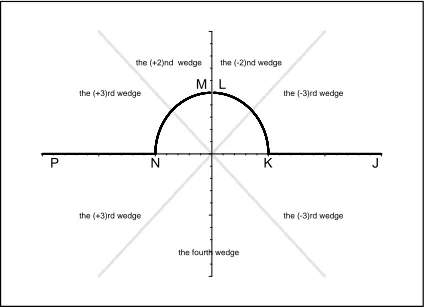
the (+3)rd wedge the (-3)rd wedge
the (+3)rd wedge the (-3)rd wedge
the fourth wedge the (-2)nd wedge the (+2)nd wedge
M L
P N K J
Figure 5. The beginning (J-K-L) and the end (M-N-P) of the unrectified tobogganic curve lying on the second Riemann sheet. The upwards-running cut starts at the origin; arbitrary units.
(±1)st Stokes wedges of Fig.4or in the (±3)rd Stokes wedges of Fig.5) or atc−= 0 (this takes place either in the zeroth and (±2)nd Stokes wedges of Figs. 4 and 5 or in the last, (+4)th = (−4)th Stokes wedge of Fig.5).
Let us assume, in addition, that the Riemann surfaceRof analyticity of our eligible physical wave functions ψ(+)(x) = e+x2
/2+O(x) or ψ(−)(x) = e−x2
/2+O(x) is just two-sheeted, i.e., that
near the origin we have ψ(x)∼xJ/2 with an odd integerJ.
For the sake of definiteness, we may pick up angular momentumℓ= 1/2 givingJ = 3. Then, the elementary change of variables ix = (iy)2 (with full details either easily derived or taken, say, from [32]) gives the new, equivalent form of wave functionϕ(y) which is, by our assumption, regular or at most weakly singular in the origin. This means that the change of variablesx→y maps the two-sheeted Riemann surface2 R onto the single ‘target” complex plane C of Fig. 6 which, formally, plays the role of a single-sheeted Riemann surface of the new, “Sturmianic” [42] wave functionϕ(y).
By construction of our particular illustrative example, there are no singularities and no cuts in the latter complex plane. For the sake of simplicity the boundaries of the Stokes wedges were also omitted in Fig.6 since they only prove relevant in the asymptotic domain where |y| → ∞.
2
Figure 6. Complexy-plane and the planarized triplet ofx-paths of Figs.4and5.
6.2 The planarizable supersymmetric toboggans
Once we return, in a climax of our preceding QTM-related exposition and considerations, to the problem of the possible SUSY partnership between strongly singular potentials, we may now feel confident that the formalism is prepared for the rigorous regularization treatment of the changes of the strength of the singularities in the potentials.
For the sake of definiteness let us start from equation (1) and assume that the generic analytic wave functionsψ(r) of the quantum system in question exhibit a general power-law behavior in the origin,
ψ(γ)0 (r)≈rγ+1/2, |r| ≪1, γ ∈R.
This implies that the related Riemann surfaceRwill be multisheeted in general, andK-sheeted (withK =K(γ)<∞) for specialγ = rational. This is one of the facts which make the problem of QTM spectra rather nontrivial in general, and this is also one of the reasons why we decided to pay here attention to the models with finiteK(γ). These models find a natural rectification-transformation regularization which eliminates the branch point(s) and “planarizes” the model in the way explained above.
In any case, our “calligraphic-font” superpotential of equation (1) acquires now one of the most elementary singular forms,
W(r) =W(γ)(r) =−∂rψ (γ) 0 (r)
ψ0(γ)(r) =χ(r)−
γ+ 1/2
r , (7)
where χ(r) may be an arbitrary function which is sufficiently regular in the origin. Thus, we know the doublet of operators A = ∂q+W and B = −∂q+W and easily deduce the explicit form of the “upper” and “lower” sub-Hamiltonians in equation (2),
H(U)=B·A= ˆp2+W2− W′, H(L)=A·B = ˆp2+W2+W′.
Near the origin, their dominant parts read as follows,
H(U)= ˆp2+ γ
2−1/4
r2 +O
1 r
, H(L)= ˆp2+(γ+ 1)
2−1/4
r2 +O
1 r
.
c(0) c(1) c(2) c(3) c(4)
d(0) d(1) d(2) d(3)
c(0) d(0) c(1) d(1) c(2) d(2)
b(0) b(1) b(2) b(3)
a(0) a(1) a(2) a(3) a(4) a(5)
-2 -1 0 1
γ
E
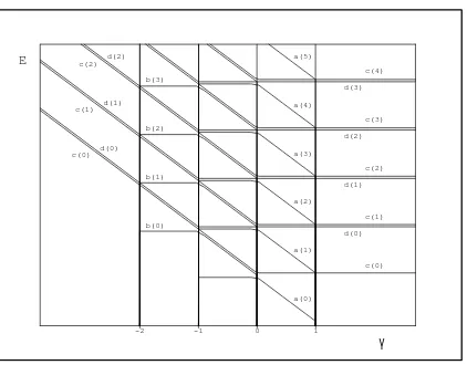
Figure 7. The γ-dependence of the spectrum of the supersymmetric model which is generated by the singular superpotential (7) whereχ(r) =r.
the winding number N), both of the SUSY-partner QTM operators may be made regular and planar (=planarized) simultaneously.
An important remark should be added here since for the realγ we haveH(U)andH(L)which depend on the mere absolute values of |γ|and|γ+ 1|, respectively. This implies the emergence of various interesting structures and asymmetries in the spectra. Some of them were described, in [24], via the exactly solvable model with linear χ(r) =r. Some of the other features of this harmonic-oscillator-like solvable toy model were discussed in proceedings [43]. Unfortunately, due to an error in printing, the illustrative spectrum did not appear in the paper. Fortunately, this information has not lost its appeal with time so we now present it via Fig.7 at last. What we see in this picture are
1) the “far left” energies which are completely degenerate,
EN(U) [≡c(N)] =EN(L) [≡d(N)], γ ∈(−∞,−2);
2) the “near left” energy levels withγ ∈(−2,−1), exhibiting a Jevicki–Rodrigues-like break-down of SUSY [2] since the new levels EN(L) [≡b(N)] remain non-degenerate;
3) the “central-domain” levels with γ ∈(−1,0),
EN(U)[≡a(N)]< EN(L)[≡b(N)] =EN(U)[≡c(N)]< EN(L)[≡d(N)] =a(N + 1)<· · ·.
Note that one obtains the usual harmonic oscillator atγ =−1/2, plus its smooth extension which ceased to be equidistant – still, the SUSY is unbroken;
4) the “near right” domain of γ∈(0,1) where the seriesEN(L) [≡b(N)] ceases to exist;
5) the “far right” spectrum with γ ∈(1,∞) and degeneracy
E(L)(+α) [≡c(N)] =d(N −1), N >0.
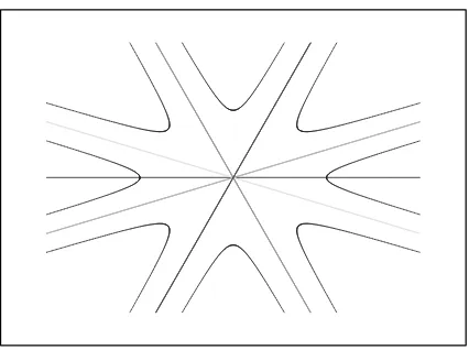
Figure 8. A sample of the planarized system of the eight QTM trajectories ofy∈ TnCˆ(s).
The sequence of the individual mapsTCˆ(s),T2Cˆ(s),T3Cˆ(s),. . .may be represented, schemat-ically, by the hyperbolas in Fig. 8 where we assumed that the whole QTM system has been planarized (i.e., there is no cut). Obviously, this picture strongly suggests that the quantitative analysis of the spectra will probably exhibit a growing difficulty with the growth of the index K(γ) = 0,1, . . . which characterizes a “hidden” topology and symmetry of the QTM system.
7
Conclusions
In the mathematical language of operator theory on can say that the QTM (or, if you wish, also PT-symmetric and other) Hamiltonians are similar to Hermitian operators [44]. In the literature one might find a lot of rigorous results in this direction (pars pro totolet us mention the brief note by Langer and Tretter [45] from 2004).
In the equally rigorous language of integrable models, the knowledge and an appropriate reinterpretation of the IM/ODE correspondence did even provide one of the most valuable proofs of reality of the spectra from H6=H† (cf. [10]).
Incidentally, the similar though much easier (and, hence, less often cited) proofs of the reality of spectra also emerged in the domain of the (new) exactly solvable models – systematic study [46] may be read as a collection of examples with further references.
On a purely heuristic level one of the most efficient formal features of the candidatesH 6=H† for Hamiltonians must be seen in theirPT-symmetry, i.e., in the peculiar intertwining property H†P =PH whereP is, unexpectedly often, an operator of (spatial) parity.
One should not forget that the boom of interest inPT-symmetric models grew even beyond the boundaries of quantum theory, viz, to various non-quantum applications of toy models H 6=H† in magnetohydrodynamics (cf. G¨unther et al. [47]) or in optics (R¨uter et al. [48]) etc.
In a parallel recent history of development of the purely pragmatic use of the concepts of supersymmetry in Quantum Mechanics (cf., e.g., [24]) one may notice the existence of the regular turns of emphasis from the appeal of the underlying algebra of operators to the necessity of studying the spaces of wave functions and the related boundary conditions. In this sense we consider the possibility of construction of SUSY QM models as systems living on topologically nontrivial Riemann surfaces [19] most appealing.
In summary, the present innovative use of the complexified coordinatesx (or y) and of the non-standard, non-Hermitian operators in SUSY context may be expected to throw new light on the multiple connections between the abstract algebras (sampled by SUSY) and nonlinear symmetries (sampled here by PT-symmetry), especially in their concrete transparent represen-tations in terms of the ordinary differential operators.
Needless to add that our text still left multiple questions entirely open. Still, some of these questions (ranging from the abstract theories down to very concrete estimates and calculations) cannot remain unanswered in a long perspective, provided that we wish to employ the proposed concepts in a more concrete phenomenological context. For this purpose we expect that the future research will move towards a deeper synthesis of the algebraic study of the foundations of SUSY QM with the truly analytic-function approaches to the mathematical as well as physical puzzles connected with the models living on more than one sheet of a Riemann surface of the (presumably, analytic) wave functions.
A
Hilbert spaces endowed with nontrivial inner products
Among applications of quantum theory one only rarely encounters unusual models like, e.g., the quantum clock in which the quantum observable is the time [49]. The wealth of possibilities offered by the abstract formalism is disproportionately often reduced just to the description of the one-dimensional motion of a point (quasi)particle. The measurement is then understood to be the measurement of positionxwhile the evolution of the wave functionψ(x) in time is assumed controlled (i.e., generated) by the Hamiltonian H = −d2/dx2 +V(x) where H
0 = −d2/dx2 represents kinetic energy and where a real function V(x) mimics the effects of an external medium.
In such a context Bender and Boettcher [6] evoked a lot of discussions by considering a one-parametric set of purely imaginary functions V(δ)(x) =x2(ix)δwith arbitrary realδ≥0 and by disentangling, simultaneously, any connection between the measurable values of position q ∈R and the admissible values of the variable x∈ C(s) inψ(x). Here, the real parameters∈R just parametrized anad hoccomplex curve such thatC(s)6=Rin general (cf., e.g., review paper [13] for more details).
In such a setting the concept of quantum toboggans has been introduced by the mere re-placement of conditionC(s)∈Cby conditionC(s)∈ Rwhere symbolRrepresents a nontrivial, multisheeted Riemann surface pertaining to wave functions ψ(x). In this case the curves C(s) may be spiral-shaped (hence the name), and only their topology must be compatible with the domains of analyticity of the underlying time-independent Schr¨odinger equation
Hψ(x) =Eψ(x), H=− d 2
dx2 +V(x)b, x∈ C(s)⊂C, s∈R. (8)
For any practical (e.g., phenomenological) purposes one then has the full freedom of making use of the analyticity properties of V(x) and ψ(x). Strictly in the spirit of [6] (or even of the older futuristic remark [50]) one may really convertthe same differential equation (8) intomany non-equivalent spectral problems by the mere variation of the underlying (classes of) curves
C(s)∈ R.
Both these questions were already addressed, in the context of nuclear physics, by Scholtz et al. [39]. In the similar, albeit more realistic physical setting these authors immediately realized that whenever one has, in the usual mathematical sense, H 6= H†, one has to leave the corresponding “usual” Hilbert-space representation L2 of the states (based on the use of the “usual” inner product hφ|ψi =R
Rφ
∗(x)ψ(x)dx) by a non-equivalent, adapted, “standard”
Hilbert-space representation denoted, say, by the symbol H(S) according to our recent brief review [15].
In the spirit of the abstract quantum theory the use of the latter space H(S) returns us to the textbook quantum theory. In particular, this space must render our given Hamilto-nian self-adjoint, i.e., it must be endowed by an amended, “metric-dependent” inner product,
hφ|ψi → hφ|Θ|ψi. The Hilbert-space-metric operator Θ itself must satisfy a certain set of natural
mathematical requirements of course [39].
Starting from the very early applications of the latter idea people often tried to avoid the direct use of the correct physical space H(S) endowed with the nontrivial metric Θ. Indeed the work within this space requires not only a suitable modification of the related Dirac-notation conventions (in this respect we shall follow here the recommendations given in [15]) but also a mind-boggling necessity of using the following “corrected” definition of the Hermitian conju-gation:
T : |ψi → hhψ|:=hψ|Θ. (9)
A comparatively easy insight in this rule is obtained when one factorizes Θ = Ω†Ω and replaces the physical spaceH(S) of kets|ψi and (doubled) brashhψ|by its unitarily equivalent “partner” Hilbert spaceH(P) of kets
|ψ(P)i:=|ψ≻:= Ω|ψi
and of bras
hψ(P)|:=≺ψ|:=hhψ|Ω−1.
On a purely abstract level of thinking one might appreciate that insideH(P)the metric is trivial again, Θ(P) =I. At the same time the price for simplification is too high in general since the Hamiltonian itself acquires a prohibitively complicated transformed form h= ΩHΩ−1.
We may summarize that in the majority of applications of models with apparent non-Hermiticity rule H 6=H† valid inside the “friendly” but “false” space L2 ≡ H(F), the concrete form of the above mentioned “non-unitary Fourier” [5] or “Dyson’s” [39] mapping Ω6= (Ω†)−1 is both ambiguous and virtually impossible to construct. A persuasive confirmation of this generic rule may be found in [51] where, up to the third order perturbation corrections,allof the eligible operators Ω were constructed for the “small” imaginary cubic potential V(x) =λix3.
It is worth adding that the ambiguity of the “admissible” metric operators Θ = Θ(H) rep-resents in fact a very unpleasant feature of the theory. For this reason, its entirely general factorization Θ = Ω†Ω in terms of the so called Dyson’s mappings Ω [39] is quite often being reduced and replaced by its more specific and less general forms3.
B
The three-Hilbert-space formulation
of quantum mechanics for quantum toboggans
On the overall background of the three-Hilbert-space formulation of quantum mechanics as given in [15] we should emphasize, at the very beginning, that there exist many important technical
3
To name just a few let us recollect the parity-using factorizations Θ =CP (= the most popular ansatz using a “charge” C such that C2
= I, cf. [9]) and Θ = PQ (where Q denotes quasi-parity, cf. [7]) – or simply the square-root factorization Θ =̺2
details of its presentation which will vary with the assumptions concerning the spectral properties of the operators in question. For this reason let us reduce the corresponding rigorous discussion to the necessary minimum and assume that all of the operators of our present interest possess just the point spectrum (composed of a finite or countably infinite number of eigenvalues and bounded from below) and no continuous or residual spectrum.
This assumption will certainly help us to simplify also the language and to use just the “minimally” modified version of the standard Dirac’s notation as described in more detail in [15]. In particular, let us recollect that the triple possibility of representation of the ket vectors may be summarized in the following, manifestly time-dependent picture inspired by the very first proposal and application [39] of the whole, and very original, scheme in nuclear physics,
physical H(P) (f ermions) difficult |ψ(t)≻ ≡ Ω(t)|ψ(t)i
Dyson′s map Ω(t) ր ց map Ω−1(t)
friendlier H(F) (bosons)
|ψ(t)i= computable
map ΩΩ−1
=I
−→ standard H(S) (bosons) |ψ(t)i the same
In this context the key innovation was twofold. Firstly, the Fourier-like mapping Ω (proposed, presumably, by Dyson) was allowed to be non-unitary. Secondly, the following arramengement of the triplet of related, Hilbert-space-dependent bra vectors proved rather unusual, showing
physical ≺ψ(t)| ∈ H(P)′
= prohibitively complicated
map Ω†(t) ր ց map Ω(t)
hψ(t)| ∈ H(F)′
= inconsistent physics
map Θ(t)=Ω†Ω6=I
−→ hhψ(t)| ∈ H(S)
′
= innovated conjugation
Two conclusions may be deduced. Firstly, the mappingT :hψ| → hhψ|=hψ|Θ may be perceived as a “very natural and very physical” or “amended” Hermitian conjugation (reason: the Hamil-tonian s made self-adjoint in H(S)). Secondly, the “double-bra” vectors may be constructed as eigenvectors of the no-metric-conjugate H† (which differs from H itself). Then, one can reconstruct the metric using the explicit formula
Θ =X|ψiihhψ|.
B.1 The hermitized “generalized eigenvalue problems” (W 6=I)
Inside the constructively inaccessible “paternal”, physical Hilbert spaceH(P) our Sturm–Schr¨ o-dinger equation is self-adjont,
h|λ≻=λ w|λ≻.
Inside the same space we may work with the Sturmianic orthogonality relations
≺λ|w|λ′≻=≺λ|w|λ≻ ·δλ,λ′
and with the Sturmianic completeness relations,
I =X λ
|λ≻ 1
In the same manner there exists the following Sturmianic spectral representation of the
Hamil-As long as the manifestly unphysical and “false” Hilbert space H(F) is still, by assumption, maximally “friendly” to computations, it makes sense to translate the above-listed formulae to this space as well. Thus, one arrives at the orthogonality relations in H(F),
hλ|Ω†wΩ|λ′i=hλ|ΘW|λ′i=hλ|ΘW|λi · δλ,λ′
as well as at the following completeness relations inside H(F),
I =X λ
|λi 1
hλ|ΘW |λihλ|ΘW.
Thirdly, the spectral decomposition of the Hamiltonian in H(F) has the following form,
H =X λ
W|λi λ
hλ|ΘW |λihλ|ΘW.
Although the choice of the convention |λii = Θ|λi represents just one of many alternative possibilities, its preference also simplifies the normalization of the overlap hλ|ΘW|λi= 1.
B.3 ΘW stays positive def inite
It is necessary to keep in mind that the use of the formal abbreviations
|ψ}=W |ψi, |ψ}}=W†|ψii
may perceivably simplify our formulae. First, it leads to an amended orthogonality,
hλ|ΘW|λ′i={{λ|λ′i=hhλ|λ′}=δλ,λ′.
Second, the alternative completeness relations read
I =X
represent, this time, not only the Hamiltonians but also the weight-operators.
In a final step of our review of the formalism we may rewrite the Dieudonn´e equations in the form
and easily derive the final single-series spectral formula
Θ =X
λ
|λii {{λ|
C
Imaginary cubic toboggans
in the large-
L
perturbation regime
For readers interested in the practical and phenomenological aspects of our present considera-tions let us briefly recall the results of calculaconsidera-tions [40] where the popular [51] non-Hermitian potentialV(x) =ix3 has been studied in the QTM kinematical regimeandin the high-angular-momentum dynamical domain.
First, the rectification change of variables did lead to the Schr¨odinger (or rather Sturm– Schr¨odinger) bound-state problem
where N is a small integer whileL is only assumed real and (very) large. We are returning to these results because they very well illustrate not only the method (of asymptotic estimates) but also the comparatively friendly nature of the spectral consequences of the topological non-triviality of the QTM integration pathsC=C(N)where, roughly speaking, the small and positive integerN is a winding number of the tobogganic path.
C.1 The method: 1/L series at N = 0 (L= ℓ, y =q(0))
Near a (local as well as global) minimumVeff(Q) of any sufficiently smooth functionVeff(q) we may often work just with the truncated forms of the Taylor series
Veff(q) =Veff(Q) +
where ξ=q−Qand where we showed in [40] that for the imaginary cubic oscillators one may select 2ℓ(ℓ+1) = 3iQ5= large and restrict the set of all of the available (complex) rootsQ=Qj, j= 1,2, . . . ,5 just to thej= 1 preferred item. Then we deduced
Lemma 1. In the non-tobogganic case the low-lying imaginary-cubic spectrum is prescribed by the estimate
leading to the leading-order harmonic-oscillator Schr¨odinger equation
C.2 The conclusion: the spectrum is N-dependent
Once we introduce T =Tj(L) as a set of roots of the elementary algebraic equation
2L(L+ 1) = (2N+ 1)2(10N + 3)T10N+5
Theorem 2. In the tobogganic cases numbered by the winding number N the low-lying imagi-nary-cubic spectrum is prescribed by the estimate
En[N]=−10N + 5
Proof . The use of the standard methods gives
Veff(y) =−
and the closed formula for the energies follows.
In terms of a parameter ρ = 1/(ℓ+ 1/2)2 our approximate spectrum may be also rescaled giving the functionFn(N)=ρ3/5En(N)with the smooth andρ-dependence which remains bounded even in the infinitely-large-ℓlimit. This is illustrated by Fig. 9 (units omitted as inessential).
–4.5 –4 –3.5 –3 –2.5 –2
0 0.0002
n (N)
F
ρ
Figure 9. The rescaled tobogganic energiesFn(N)=ρ3/5En(N)(ρ) in the imaginary cubic well. The first
four lowest energies with n= 0,1,2,3 are sampled at very small ρ= 1/(ℓ+ 1/2)2. The increase of the
winding N = 0,1, . . . ,8 pushes the spectrum downwards.
–800 –700 –600 –500 –400
0.0001 0.0002
n (N)
E
ρ
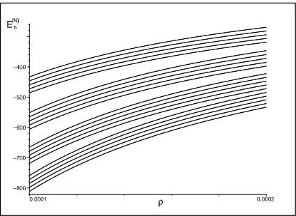
Figure 10. The unrescaled tobogganic energies En(N)(ρ) in the imaginary cubic well. The first five
lowest energies with n= 0,1,2,3,4 are sampled in a non-asymptotic interval ofρ > ρ0>0. The result
is shown for windingsN = 0,1,2 and 3.
Acknowledgements
Work supported by MˇSMT “Doppler Institute” project Nr. LC06002, by the GA ˇCR grant Nr. P203/11/1433, by the Institutional Research Plan AV0Z10480505 and, last but not least, by the hospitality of STIAS in Stellenbosch in November 2010.
References
[1] Cooper F., Khare A., Sukhatme U., Supersymmetry and quantum mechanics,Phys. Rep.251(1995), 267–
385,hep-th/9405029.
[2] Jevicki A., Rodrigues J.P., Singular potentials and supersymmetry breaking, Phys. Lett. B 146 (1984),
55–58.
[3] Junker G., Supersymmetric methods in quantum and statistical physics,Text and Monographs in Physics, Springer-Verlag, Berlin, 1996.
Bagchi B.K., Supersymmetry in quantum and classical mechanics,Chapman&Hall/CRC Monographs and Surveys in Pure and Applied Mathematics, Vol. 116, Chapman & Hall/CRC, Boca Raton, FL, 2001.
[5] Buslaev V., Grecchi V., Equivalence of unstable anharmonic oscillators and double wells,J. Phys. A: Math. Gen.26(1993), 5541–5549.
Andrianov A.A., Ioffe M.V., Cannata F., Dedonder J.-P., SUSY quantum mechanics with complex super-potentials and real energy spectra,Internat. J. Modern Phys. A14(1999), 2675–2688,quant-ph/9806019.
Cannata F., Junker G., Trost J., Schr¨odinger operators with complex potential but real spectrum, Phys.
Lett. A246(1998), 219–226,quant-ph/9805085.
Bender C.M., Boettcher S., Meisinger P.M.,PT-symmetric quantum mechanics,J. Math. Phys.40(1999),
2201–2229,quant-ph/9809072.
[6] Bender C.M., Boettcher S., Real spectra in non-Hermitian Hamiltonians havingPT symmetry,Phys. Rev.
Lett.80(1998), 5243–5246,physics/9712001.
[7] Znojil M., Conservation of pseudo-norm inPT symmetric quantum mechanics,math-ph/0104012.
[8] Mostafazadeh A., Pseudo-Hermiticity versusPT Symmetry: the necessary condition for the reality of the spectrum of a non-Hermitian Hamiltonian,J. Math. Phys.43(2002) 205–214,math-ph/0107001.
Mostafazadeh A., Pseudo-Hermiticity versus PT-symmetry. II. A complete characterization of non-Hermitian Hamiltonians with a real spectrum,J. Math. Phys.43(2002), 2814–2816,math-ph/0110016.
Mostafazadeh A., Pseudo-Hermiticity versusPT-symmetry. III. Equivalence of pseudo-Hermiticity and the presence of antilinear symmetries,J. Math. Phys.43(2002), 3944–3951,math-ph/0203005.
[9] Bender C.M., Brody D.C., Jones H.F., Complex extension of quantum mechanics, Phys. Rev. Lett. 89
(2002), 270402, 4 pages, Erratum,Phys. Rev. Lett.92(2004), 119902, 1 page,quant-ph/0208076.
[10] Dorey P., Dunning C., Tateo R., Spectral equivalences, Bethe ansatz equations, and reality properties in
PT-symmetric quantum mechanics,J. Phys. A: Math. Gen.34(2001), 5679–5704,hep-th/0103051.
[11] Znojil M., Comment on: “Supersymmetry and singular potentials” by Das and Pernice [Nuclear Phys. B 561(1999), 357–384],Nuclear Phys. B662(2003), 554–562,hep-th/0209262.
[12] Dorey P., Dunning C., Tateo R., The ODE/IM correspondence,J. Phys. A: Math. Theor.40(2007), R205–
R283,hep-th/0703066.
[13] Bender C.M., Making sense of non-Hermitian Hamiltonians, Rep. Progr. Phys. 70 (2007), 947–1018, hep-th/0703096.
[14] Mostafazadeh A., Pseudo-Hermitian representation of quantum mechanics, Int. J. Geom. Methods Mod.
Phys.7(2010), 1191–1306,arXiv:0810.5643.
[15] Znojil M., Three-Hilbert-space formulation of quantum mechanics, SIGMA 5 (2009), 001, 19 pages, arXiv:0901.0700.
[16] Znojil M., PT-symmetric regularizations in supersymmetric quantum mechanics,J. Phys. A: Math. Gen.
37(2004), 10209–10222,hep-th/0404145.
[17] Znojil M.,PT-symmetric quantum toboggans,Phys. Lett. A342(2005), 36–47,quant-ph/0502041.
[18] Fern´andez F.M., Guardiola R., Ros J., Znojil M., A family of complex potentials with real spectrum,
J. Phys. A: Math. Gen.32(1999), 3105–3116,quant-ph/9812026.
Znojil M., Spiked potentials and quantum toboggans, J. Phys. A: Math. Gen. 39 (2006), 13325–13336, quant-ph/0606166.
Novotn´y J.,http://demonstrations.wolfram.com/TheQuantumTobogganicPaths/.
[19] Znojil M., Jakubsk´y V., Supersymmetric quantum mechanics living on topologically nontrivial Riemann surfaces,Pramana J. Phys.73(2009), 397–404,arXiv:0904.2294.
[20] Correa F., Jakubsk´y V., Nieto L.M., Plyushchay M.S., Self-isospectrality, special supersymmetry, and their effect on the band structure,Phys. Rev. Lett.101(2008), 030403, 4 pages,arXiv:0801.1671.
Correa F., Jakubsk´y V., Plyushchay M.S., Finite-gap systems, tri-supersymmetry and self-isospectrality,
J. Phys. A: Math. Theor.41(2008), 485303, 35 pages,arXiv:0806.1614.
Siegl P., Supersymmetric quasi-Hermitian Hamiltonians with point interactions on a loop,J. Phys. A: Math.
Theor.41(2008), 244025, 11 pages.
Jakubsk´y V., Nieto L.M., Plyushchay M.S., Klein tunneling in carbon nanostructures: a free-particle dy-namics in disguise,Phys. Rev. D63(2011), 047702, 4 pages,arXiv:1010.0569.
[21] Andrianov A.A., Cannata F., Sokolov A.V., Non-linear supersymmetry for Hermitian, non-diagonalizable Hamiltonians. I. General properties,Nuclear Phys. B773(2007), 107–136,math-ph/0610024.
[23] Znojil M., PT symmetrized SUSY quantum mechanics, Czechoslovak J. Phys. 51 (2001), 420–428, hep-ph/0101038.
Znojil M.,PT-symmetry and supersymmetry, in GROUP 24: Physical and Mathematical Aspects of Sym-metries (Paris, July 15–20, 2002), IOP Publishing, Bristol, 2003, 629–632,hep-th/0209062.
[24] Znojil M., Non-Hermitian SUSY and singular, PT-symmetrized oscillators, J. Phys. A: Math. Gen. 35
(2002), 2341–2352,hep-th/0201056.
[25] Levai G., Znojil M., The interplay of supersymmetry and PT symmetry in quantum mechanics: a case study for the Scarf II potential,J. Phys. A: Math. Gen.35(2002), 8793–8804,quant-ph/0206013.
Sinha A., Roy P., Generation of exactly solvable non-Hermitian potentials with real energies,Czechoslovak
J. Phys.54(2004), 129–138,quant-ph/0312089.
[26] Caliceti E., Graffi S., Maioli M., Perturbation theory of odd anharmonic oscillators,Comm. Math. Phys.
75(1980), 51–66.
Sibuya Y., Global theory of second order linear differential equation with polynomial coefficient, North Holland, Amsterdam, 1975.
Fern´andez F.M., Guardiola R., Ros J., Znojil M., Strong-coupling expansions for thePT-symmetric oscil-latorsV(r) =aix+b(ix)2
+c(ix)3
,J. Phys. A: Math. Gen.31(1998), 10105–10112.
[27] Znojil M.,PT-symmetric harmonic oscillators,Phys. Lett. A259(1999), 220–223.
[28] Znojil M.,PT-symmetric square well,Phys. Lett. A285(2001), 7–10,quant-ph/0101131.
Quesne C., Bagchi B., Mallik S., B´ıla H., Jakubsk´y V., Znojil M., PT-supersymmetric partner of a short-range square well,Czechoslovak J. Phys.55(2005), 1161–1166,quant-ph/0507246.
[29] Albeverio S., Fei S.-M., Kurasov P., Gauge fields, point interactions and few-body problems in one dimension,
Rep. Math. Phys.53(2004), 363–370,quant-ph/0406158.
[30] Znojil M., Tater M., Complex Calogero model with real energies,J. Phys. A: Math. Gen.34(2001), 1793–
1803,quant-ph/0010087.
Znojil M., Low-lying spectra in anharmonic three-body oscillators with a strong short-range repulsion,
J. Phys. A: Math. Gen.36(2003), 9929–9941,quant-ph/0307239.
Fring A., Smith M., Antilinear deformations of Coxeter groups, an application to Calogero models,
J. Phys. A: Math. Theor.43(2010), 325201, 28 pages,arXiv:1004.0916.
[31] Znojil M., Quantum knots,Phys. Lett. A372(2008), 3591–3596,arXiv:0802.1318.
[32] Znojil M., Quantum toboggans: models exhibiting a multisheeted PT symmetry,J. Phys. Conf. Ser.128
(2008), 012046, 12 pages,arXiv:0710.1485.
[33] Wessels G.J.C., A numerical and analytical investigation into non-Hermitian Hamiltonians, Master Thesis, University of Stellenbosch, 2008.
[34] B´ıla H., Spectra of PT-symmetric Hamiltonians on tobogganic contours, Pramana J. Phys. 73 (2010),
307–314,arXiv:0905.1498.
[35] Dorey P., Millican-Slater A., Tateo R., Beyond the WKB approximation inPT-symmetric quantum me-chanics,J. Phys. A: Math. Gen.38(2005), 1305–1331,hep-th/0410013.
[36] Znojil M., Quantum toboggans with two branch points,Phys. Lett. A372(2008), 584–590,arXiv:0708.0087.
[37] Znojil M., Classification of oscillators in the Hessenberg-matrix representation,J. Phys. A: Math. Gen.27
(1994), 4945–4968.
[38] Znojil M., Siegl P., Levai G., Asymptotically vanishing PT-symmetric potentials and negative-mass Schr¨odinger equations,Phys. Lett. A373(2009), 1921–1924,arXiv:0903.5468.
[39] Scholtz F.G., Geyer H.B., Hahne F.J.W., Quasi-Hermitian operators in quantum mechanics and the varia-tional principle,Ann. Physics213(1992), 74–101.
[40] Znojil M., Topology-controlled spectra of imaginary cubic oscillators in the large-Lapproach,Phys. Lett. A
374(2010), 807–812,arXiv:0912.1176.
[41] Znojil M., Gemperle F., Mustafa O., Asymptotic solvability of an imaginary cubic oscillator with spikes,
J. Phys. A: Math. Gen.35(2002), 5781–5793,hep-th/0205181.
[42] Znojil M., Identification of observables in quantum toboggans,J. Phys. A: Math. Theor.41(2008), 215304,
14 pages,arXiv:0803.0403.
Znojil M., Geyer H.B., Sturm–Schr¨odinger equations: formula for metric, Pramana J. Phys. 73 (2010),
299–306,arXiv:0904.2293.
[44] Dieudonn´e J., Quasi-Hermitian operators, in Proc. Internat. Sympos. Linear Spaces (Jerusalem, 1960), Pergamon, Oxford, 1961, 115–122.
Williams J.P., Operators similar to their adjoints,Proc. Amer. Math. Soc.20(1969), 121–123.
[45] Langer H., Tretter Ch., A Krein space approach toPT-symmetry,Czechoslovak J. Phys.54(2004), 1113–
1120.
[46] L´evai G., Znojil M., Systematic search forPT-symmetric potentials with real energy spectra,J. Phys. A:
Math. Gen.33(2000), 7165–7180.
[47] G¨unther U., Langer H., Tretter Ch., On the spectrum of the magnetohydrodynamic mean-fieldα2
-dynamo operator,SIAM J. Math. Anal.42(2010), 1413–1447,arXiv:1004.0231.
Znojil M., G¨unther U., Dynamics of charged fluids and 1/ℓperturbation expansions, J. Phys. A: Math.
Theor.40(2007), 7375–7388,math-ph/0610055.
[48] R¨uter C.E., Makris K.G., El-Ganainy R., Christodoulides D.N., Segev D.N., Kip D., Observation of parity-time symmetry in optics,Nature Phys.6(2010), 192–195.
Berry M.V., Optical lattices withPT symmetry are not transparent, J. Phys. A: Math. Theor.41(2008),
244007, 7 pages.
Makris K.G., El-Ganainy R., Christodoulides D.N., Musslimani Z.H., Beam dynamics in PT symmetric optical lattices,Phys. Rev. Lett.100(2008), 103904, 4 pages.
[49] Hilgevoord J., Time in quantum mechanics,Amer. J. Phys.70(2002), 301–306.
[50] Bender C.M., Turbiner A., Analytic continuation of eigenvalue problems,Phys. Lett. A173(1993), 442–446.
[51] Mostafazadeh A., Metric operator in pseudo-Hermitian quantum mechanics and the imaginary cubic poten-tial,J. Phys. A: Math. Gen.39(2006), 10171–10188,quant-ph/0508195.
[52] Jones H.F., Mateo J., Equivalent Hermitian Hamiltonian for the non-Hermitian−x4
potential,Phys. Rev. D
73(2006), 085002, 4 pages,quant-ph/0601188.
Bagchi B., Fring A., Minimal length in quantum mechanics and non-Hermitian Hamiltonian systems,Phys.