CARTESIAN DIFFERENTIAL CATEGORIES
R.F. BLUTE, J.R.B. COCKETT AND R.A.G. SEELY
Abstract. This paper revisits the authors’ notion of a differential category from a different perspective. A differential category is an additive symmetric monoidal category with a comonad (a “coalgebra modality”) and a differential combinator. The morphisms of a differential category should be thought of as the linear maps; the differentiable or smooth maps would then be morphisms of the coKleisli category. The purpose of the present paper is to directly axiomatize differentiable maps and thus to move the emphasis from the linear notion to structures resembling the coKleisli category. The result is a setting with a more evident and intuitive relationship to the familiar notion of calculus on smooth maps. Indeed a primary example is the category whose objects are Euclidean spaces and whose morphisms are smooth maps.
ACartesiandifferential category is a Cartesian left additive category which possesses a Cartesian differential operator. The differential operator itself must satisfy a number of equations, which guarantee, in particular, that the differential of any map is “linear” in a suitable sense.
We present an analysis of the basic properties of Cartesian differential categories. We show that under modest and natural assumptions, the coKleisli category of a differential category is Cartesian differential. Finally we present a (sound and complete) term calculus for these categories which allows their structure to be analysed using essentially the same language one might use for traditional multi-variable calculus.
0. Introduction
Over the past few centuries, one of the most fundamental concepts in all of mathematics has been differentiation. In recent decades several attempts have been made to abstract this notion, including approaches based on geometric, algebraic, and logical intuitions. The approach of the current paper is categorical, insofar as we wish to consider axiom-atizations of categories which have sufficient structure to define differentiation of maps. Any additional categorical structure, e.g. monoidal, Cartesian, or comonadic, exists in support of differentiation.
In [BCS 06], the current authors introduced the notion of a differential category to provide a basic axiomatization for differential operators in monoidal categories. The initial impetus for the definition came from work of Ehrhard and Regnier [Ehrhard & Regnier 05, Ehrhard & Regnier 03], who defined first a notion of differential λ-calculus
Received by the editors 2008-11-29 and, in revised form, 2009-12-08. Transmitted by Robert Par´e. Published on 2009-12-10.
2000 Mathematics Subject Classification: 18D10,18C20,12H05,32W99.
Key words and phrases: monoidal categories, differential categories, Kleisli categories, differential operators.
c
R.F. Blute, J.R.B. Cockett and R.A.G. Seely, 2009. Permission to copy for private use granted.
and subsequently differential proof nets. The differential λ-calculus is an extension of simply-typedλ-calculus with an additional operation allowing the differentiation of terms. Differential proof nets are a (graph-theoretic) syntax for linear logic extended with a differential operator on proofs. An important feature of their systems, not precluded in ours, is that in one setting, they combine the essence of both calculus and computability. Their work grew out of the development of models of linear logic (examples of ∗ -autonomous categories) in which there was a natural differential operator, such as K¨othe spaces [Ehrhard 01]. Every model of linear logic comes equipped with a monad, the storage operator, from which the coKleisli category arises. One can then abstract away from models of linear logic, retaining the comonad as the key feature. From this perspective it is a very natural step to consider the coKleisli categories of such models, not least because it is this setting which supports a calculus which much more closely resembles the elementary differential calculus with which we are all familiar. The calculus one obtains from this perspective is quite different than the differential lambda-calculus of Ehrhard and Regnier, in that it is directly inspired by the coKleisli structure. And so this left open the question of how to characterize this situation.
The notion of a differential category provides a basic axiomatization for differential operators in monoidal categories, which not only generalizes the work of Ehrhard and Regnier but also captures the standard elementary models of differential calculus and provides a theoretical substrate for studying a number of less standard examples. The structure necessary to support differentiation in [BCS 06] is an additive, monoidal category with a coalgebra modality. (These terms will be reviewed below.) The morphisms in a differential category should be thought of as linear maps, with maps in the coKleisli category being the smooth maps. Then the differential operator is of the following type:
f:SA //B D⊗[f]:A⊗SA //B
One then writes down suitable axioms which such an operator must satisfy. In particular, we have the Leibniz rule, the chain rule, and other basic rules of differentiation expressed coalgebraically.
The goal of the present paper is to develop an axiomatisation which directly character-izes the smooth maps: in other words, to characterize the coKleisli structure of differential categories directly. This leads us to the notion of a Cartesian differential category. This notion embodies the multi-variable differential calculus which, being a fundamental tool of modern mathematics, is well worth studying in its own right. The basic structure needed for Cartesian differential categories is simpler than is needed for differential categories: just a left additive category with finite products. The differential operator takes on the following form
X f //Y X×X
D×[f]
/
/Y
turns out to be surprisingly subtle. While we do describe the conditions under which a differential category gives rise to a Cartesian differential category as its coKleisli category, a full characterization of this situation is left to a sequel. The main result in this direction is Proposition 3.2.1.
The organization of the paper is as follows. Fundamental to differentiation is the ability to add maps: however, the settings in which we are interested are not additively enriched. Therefore the first section is dedicated developing the general theory of left additive categories. In the second section we introduce the key notion of a Cartesian differential operator and the equations it satisfies. In this section, we also show how most of the axiomatization of these categories is determined by requiring that their “bundle categories” behave in the expected manner. These are fibrations which carry the differ-ential structure, insofar as the composition of maps is just the chain rule. It is possible to develop order bundle categories in which composition is determined by the higher-order (Fa`a di Bruno) chain rules. These higher-differential bundle categories completely determine all the axiomatization of Cartesian differential categories, but developing this would require more technical apparatus than seems justified in this paper, so will be presented elsewhere.
As always, we are interested in graphical representations of morphisms in free cate-gories, an approach begun in [BCST 97]. But in this paper we focus more on a term calculus. This calculus can be seen as effectively reimagining the traditional differential calculus as a rewrite system. Section 4 of this paper is devoted to analyzing this system in detail. In particular, we show the system’s soundness and completeness. The term calculus allows for an elegant description of free Cartesian differential categories, which we shall present in a sequel.
The reader should keep one key simple example in mind when reading the paper: the category of smooth maps, which behaves just as one would expect from a first year calculus course. Objects are natural numbers and maps n //m are smooth maps IRn //IRm.
It is easiest to describe the differential operator via an example. Suppose we have a smooth map f: 3 //1, such as f(x, y, z) =xyz. The Jacobian of this map is [yz, xz, xy] which may be regarded as a smooth operator which assigns a linear operator to any point (x, y, z). This is how we get a smooth mapD×(f):IR3×IR3 //IR, which is linear in the
first variable (in the first triple of coordinates):
D×(f): ((u, v, w),(r, s, t))7→(st, rt, rs)·(u, v, w) =stu+rtv+rsw
In fact, the notation we will introduce in our term calculus is slightly different than this, and keeps more careful track of free vs. bound variables. This leads to one of our axioms for Cartesian differential categories: the function D[f] is linear in its first n variables. The rest of the axioms express other aspects of differentiability.
turn the world of mathematics and philosophy upside down to ensure that everything be-comes differentiable. Somewhere nearer the middle is the Platonic approach which takes the view that the ability to differentiate ultimately devolves onto the topological and lim-iting properties of a single crucial object: the real line. And then there is the mechanical approach. Devoid of overarching philosophy or greater purpose, it takes calculus as a system which, like any other, should immediately be taken apart to determine how the behavior of one part depends on structure in some other part. Dismembering calculus in this manner, it seeks to reuse these structures in outlandish configurations elsewhere.
This work belongs unapologetically to this last camp. It seeks to isolate some basic structural properties which give rise to behaviors reminiscent of the differential calculus. We believe abstracting differential calculus in this manner serves a useful purpose which also reflects developments in other areas. Differentials (over arbitrary base rings) are used non-trivially in various areas of algebraic geometry, and differentials also appear in different guises in both combinatorics and computer science. A framework unifying such notions is useful, and in particular allows one to distinguish clearly between what is generic and what is specific.
1. Left additive categories
The purpose of this section is to develop the basic theory of left additive categories which underlies the theory of Cartesian differential categories. As a basic example consider the category of commutative monoids with morphisms which are arbitrary maps which ignore the additive structure. Despite the fact that additive structure is being ignored, the maps between any two objects have a natural additive structure, given by pointwise addition (f+g)(x) =f(x)+g(x). Furthermore, this additive structure is preserved by composition on the left h(f +g) = hf +hg (throughout the paper we use the diagrammatic order of composition, sometimes denoted with a semicolon, often just by juxtaposition). A category with the property that each homset is a commutative monoid and for which composition on the left preserves this structure is called a left additive category.
This category may be viewed rather differently: it is the coKleisli category with respect to the comonad generated from the comonad on commutative monoids generated by the composite of the underlying functor and the free functor. This illustrates an important way in which left additive structure arises: any (non-additive) comonad on an additive (or indeed left-additive) category always has its coKleisli category left-additive.
Another basic example of a left additive category which is central to this paper consists of the category whose objects are finite dimensional real vector spaces and whose maps are (infinitely) differentiable maps. These maps allow pointwise addition and so certainly form a left additive category. In addition, this category has a differential structure which is the main subject matter of the paper and is discussed in the next section.
1.1.1. Definition. A category X is left additive1 in case each hom-set is a
commu-tative monoid and f(g+h) = (f g) + (f h)andf0 = 0. A maph in a left additive category is said to be additiveif it also preserves the additive structure of the hom-set on the right
(f+g)h= (f h) + (gh) and 0h= 0.
In general additive maps will be the exception in a left additive category. However, the additive maps form an interesting subcategory:
1.1.2. Proposition. In any left additive category,
1. 0 maps are additive;
2. additive maps are closed under addition;
3. additive maps are closed under composition;
4. all identity maps are additive;
5. if m is an additive monic andf m is additive then f is additive;
6. if g is a retraction which is additive and the composite gh is additive then h is additive;
7. if r is a retraction with section m so that the idempotent rm is additive, then r is additive iff its section m is additive;
8. if f is an isomorphism which is additive, then f−1 is additive.
Proof. (1): (f +g)0 = 0 = 0 + 0 =f0 +g0.
(2): Iff andgare additive then (x+y)(f+g) = (x+y)f+(x+y)g =xf+yf+xg+yg= x(f+g) +y(f+g).
(3): If f and g are additive then (x+y)f g= (xf+yf)g =xf g+yf g. (4 ,5): Immediate.
(6): This is slightly more subtle: suppose g is additive and a retraction, so that there is ag′ withg′g = 1, andghis additive then, as (x+y) = (xg′g+yg′g) = (xg′+yg′)g then
(x+y)h= (xg′+yg′)gh=xg′gh+yg′gh=xh+yh.
(7): Since rm is additive, by (5) if m is additive, then r is additive; and by (6) if r is additive then m is additive.
(8): If f is an isomorphism it is certainly a retraction and 1 = f f−1 is certainly
additive so by the previous property f−1 is additive.
1We should emphasize that our “additive categories” are commutative monoid enriched categories,
Note that it is certainly not the case that all isomorphisms are additive. However, we can conclude:
1.1.3. Corollary. The additive maps of a left additive category X form an additive
subcategory whose inclusion I:X+ //X reflects isomorphisms.
1.1.4. Example. The category CMon of commutative monoids with “set maps” (i.e.
without any preservation properties) is left additive, but generally its maps are not addi-tive. Left additivity is easily shown:
f(g+h)(x) = (g+h)(f(x)) = g(f(x)) +h(f(x)) = (f g)(x) + (f h)(x) = (f g+f h)(x) (and 0 is similar). As an example of the failure of additivity, however, consider that (0f)(x) =f(0(x)) = f(0), and we have explicitly not requiredf(0) = 0 (and similarly for addition). The additive maps in this setting are just the commutative monoid homomor-phisms.
1.2. Cartesian left additive categories. Our main interest centres around left
additive categories which have products which behave coherently with respect to the additive structure:
1.2.1. Definition. A Cartesian left additive category is a left additive category
with products such that the structure maps π0, π1, and ∆ are additive and that whenever
f and g are additive then f ×g is additive.
Notice that if f and g are additive then hf, gi is additive as
(x+y)hf, gi= (x+y)∆(f×g) = x∆(f ×g) +y∆(f×g) = xhf, gi+yhf, gi
Conversely one may replace the requirement that ∆ is additive and that × preserves additivity by the single requirement that pairing preserves additivity as both can be ex-pressed by pairing additive maps. Thus, equivalently, a category is Cartesian left additive in case it has products for which the projections are additive and whenever f and g are additive then hf, gi is additive. Cartesian left additive categories can be formulated in various other ways as well:
1.2.2. Proposition. The following are equivalent:
(i) A Cartesian left additive category;
(ii) A left additive category with products such that all projections and pairings of additive maps are additive.
(iii) A left additive category for which X+ has biproducts and the the inclusionI:X+ //X
creates products;
(iv) A Cartesian category X in which each object is equipped with a chosen commutative
Proof.
(i) ⇔ (ii) Above.
(ii) ⇒ (iii) Clearly as the product structure is additive the category of additive maps will have products (and so biproducts). Further, the inclusion functor will clearly create products. Furthermore, each πi is additive as
(hf, f′i+hg, g′i)π0 =hhf, f′i,hg, g′ii(π0×π0)+ =hf, f′iπ0 +hg, g′iπ0.
Clearly maps are additive in case they are homomorphisms of the chosen additive structure: but this means if f and g are additive then hf, gi is additive as the additive structure on the product is the product additive structure!
The last characterization does rely on the choice of product structure. The equivalence to being Cartesian left additive informs us that the choice can be made up to additive isomorphism. For, seen as a left additive category, there is one global structure albeit it may be represented locally in a variety of coherent ways.
The fact that an additive map f:A // B in a Cartesian left additive category is precisely a homomorphism of the additive structure
A×A
1.2.3. Lemma. In a Cartesian left additive category:
(i) hf, gi+hf′, g′i=hf +f′, g+g′i and 0 =h0,0i;
(ii) f is additive if and only if
(π0+π1)f =π0f +π1f:A×A //B and 0f = 0: 1 //B;
(iii) g:A×X //B is additive in its second argument if and only if
1×(π0+π1)g = (1×π0)g+(1×π1)g:A×X×X //B and (1×0)g = 0:A×1 //B.
Being additive in the second argument means hx, y + zig = hx, yig + hx, zig and
hx,0ig = 0; being additive in an argument is a property which will become more central shortly.
Proof.
(i) We have the following calculation:
hf, gi+hf′, g′i = (hf, gi+hf′, g′i)hπ0, π1i
= h(hf, gi+hf′, g′i)π0,(hf, gi+hf′, g′i)π1i
= hhf, giπ0+hf′, g′iπ0,hf, giπ1+hf′, g′iπ1i
= hf+f′, g+g′i
and a similar calculation for the zero.
(ii) If f is additive this equality holds. Conversely
(h+k)f =hh, ki(π0 +π1)f =hh, ki(π0f+π1f) =hf +kf.
(iii) Similar.
One reason for demanding that the product structure be additive is the following (which uses the fact that products in additive categories are necessarily biproducts):
1.2.4. Corollary. For any Cartesian left additive category X the subcategory of the
additive maps I:X+ //X has biproducts.
Again we may consider the example CMon: it is clear that letting the product be the usual product of commutative monoids will ensure that we obtain a Cartesian left additive category. Note that an arbitrary monoid which has base set the product of the base sets of M1 and M2 will not work as the left additive product asπ0+π1 will no longer give the
1.3. Cartesian left additive functors.
1.3.1. Definition. A functor between Cartesian left additive categories is Cartesian
left additive in case
• F(f+g) =F(f) +F(g) and F(0) = 0;
• F preserves products (i.e F(A)oo F(π0) F(A×B) F(π1) //F(B) is a product). Clearly the identity functor is left additive and we may compose Cartesian left addi-tive functors, thus, this, together with natural transformations (whose components are additive) gives the data for a 2-category. Notice that Cartesian left additive functors pre-serve the additive structure maps A×A + //Aoo 0 1 so, crucially for the 2-dimensional structure, we have:
1.3.2. Lemma. A left additive functor is a Cartesian left additive functor if and only if
it preserves additive maps.
Proof. A map is additive if and only if it is a homomorphism of the given additive
structure: this property is preserved by Cartesian left additive functors. The converse follows as biproducts are equationally defined using the additive maps.
Suppose S= (S, δ, ǫ) is any comonad (whereS need not be Cartesian left additive) on a Cartesian left additive category,X. Then clearly the coKleisli mapsS(X) f //Y inherit an addition fromX and with thisXS becomes left additive. (In the following calculation, we shall distinguish maps in the coKleisli category by setting them in boldface; maps in X will be in ordinary type.)
f(g1+g2)=δS(f)(g1+g2) =δS(f)g1+δS(f)g2 =f g1+f g2
As XS is a coKleisli category it has products inherited from X with
X oo π0 X ×Y π1 //Y =Xoo ǫπ0 S(X×Y) ǫπ1 //Y. Note that these projections are additive in XS as
(f +g)π0 =δS(f+g)ǫπ0 = (f +g)π0 = (f π0) + (gπ0) =(f π0) + (gπ0)
Consider the pairing map:
Z hf,gi //X ×Y =S(Z) hf,gi //X×Y and suppose f and g are additive in XS then
(x+y)hf ,gi = δS(x+y)hf, gi=hδS(x+y)f, δS(x+y)gi
= h(x+y)f,(x+y)gi =hxf +yf, xg+ygi
= hxf, xgi+hyf, ygi=xhf, gi+yhf, gi
1.3.3. Proposition. If S = (S, δ, ǫ) is any comonad on a (Cartesian) left additive
category X then XS is (Cartesian) left additive. Furthermore the canonical right adjoint GS:X //XS is a Cartesian left additive functor.
Proof. The hard work was done above! It remains to check that GS is additive as it
clearly preserves products; for this we need
GS(f+g) =ǫ(f +g) = ǫf +ǫg =GS(f) +GS(g) and GS(0) =ǫ0 = 0.
As an application of Proposition 1.3.3, we note that since a Cartesian left additive category X has products, for each object A ∈ X the functor ×A is a comonad (using the fact that A is canonically a comonoid); the coKleisli category is sometimes known as the “simple slice category at A”; we shall denote it X[A]:
1.3.4. Definition. X[A] (called “the simple slice category at A”) has as objects the
objects ofX, and as morphismsf:X //Y morphismsf:X×A //Y of X. Identities are
given by projections, and composition is the coKleisli composition: X f //Y g //Z = X×A ∆×1 //X×A×A 1×f //Y ×A g //Z.
1.3.5. Corollary. Each simple slice X[A] of a Cartesian left additive category X is a
Cartesian left additive category.
Notice that the additive functions in X[A] are exactly the mapsf:X×A //Y which are additive in their first argument in the sense that hx+y, zif =hx, zif +hy, zif and
h0, zif = 0.
1.4. Cartesian closed left additive categories. A left additive category is a
Cartesian closed left additive categoryin case it is a Cartesian left additive category which is Cartesian closed, so A× is a left adjoint with right adjoint A ⇒ , such that the passage:
A×X f //Y X
curry(f) //A⇒Y
preserves the additive structure. That is curry(f+g) = curry(f)+curry(g) and curry(0) = 0.
1.4.1. Lemma. A Cartesian left additive category X is a Cartesian closed left additive
category if and only if X is Cartesian closed and
Proof. “Only if” is obvious by considering adjoints. For the converse, we note that when the stated condition holds we have:
curry(f+g) = curry(hf, gi)(A⇒+B)
= hcurry(f),curry(g)ik×(A⇒+B)
= hcurry(f),curry(g)i+A⇒B= curry(f) + curry(g)
so that addition is preserved by currying: the preservation of zero is similar. Thus, the category is Cartesian closed left additive.
When a category is Cartesian closed then (A⇒ , η, µ) is a monad for each objectA where
A×X π1 //X X
curry(π1)
/
/A⇒Y η
A×(A⇒(A⇒X)) ∆×1 //A×A×(A ⇒(A⇒X)) 1×eval //A×(A⇒X) eval //X A⇒(A⇒X)
curry((∆×1)(1×eval)eval) //A⇒X
µ
The Kleisli category for this monad is clearly isomorphic to X[A] and the coherence requirement for closedness ensures that the two additive structures inherited from X, regarding it as a Kleisli and coKleisli category respectively, coincide.
In particular note that in a Cartesian closed left additive category A×X f //Y is additive in its second argument if and only ifX curry(f) //A⇒Y is additive. Once again we may consider CMon: this is a Cartesian closed left additive category provided one endows the hom-sets with the pointwise additive structure f +g =λx.f(x) +g(x).
1.5. Additive bundle fibrations. Of course, there is a well-known fibration
associ-ated with the simple slice categories; we are interested in the subfibration whose fibres are just the additive parts of the simple fibres. We think of this fibration as the fibration of “additive bundles” overX, and so denote it byp: ABun(X) //X. The objects of ABun(X) are pairs (X, A), its morphisms (X, A) //(Y, B) are pairs (F, f) of morphisms ofX, where F:X×A //Y is additive in its first argument, and f:A //B. Composition is defined by (F, f)(G, g) = (hF, π1fiG, f g), and the identities are (π0,1A). We shall check (below)
that if F, G are additive in the first variable, so ishF, π1fiG.
ABun(X) has additive structure, defined coordinate-wise: (F, f)+(G, g) = (F+G, f+ g), 0 = (0,0). It also has products: 1 = (1,1) and
(X, A)oo (π0π0,π0) (X×Y, A×B) (π0π1,π1) //(Y, B) In fact:
Proof. There are a number of things to check — here are those that are not perfectly obvious.
Composition preserves additivity in the first component:
hx+y, zihF, π1fiG = hhx+y, ziF, zfiG
= hhx, ziF +hy, ziF, zfiG
= hhx, ziF, zfiG+hhy, ziF, zfiG = hx, zihF, π1fiG+hy, zihF, π1fiG
Addition is well-defined (i.e. F +Gis additive in the first variable):
hx+y, zi(F +G) = hx+y, ziF +hx+y, ziG
= hx, ziF +hx, ziG+hy, ziF +hy, ziG = hx, zi(F +G) +hy, zi(F +G)
(F +G, f +g) is left additive:
(H, h)(F +G, f +g) = (hH, π1hi(F +G), h(f+g))
= (hH, π1hiF +hH, π1hiG, hf +hg)
= (hH, π1hiF, hf) + (hH, π1hiG, hg)
= (H, h)(F, f) + (H, h)(G, g) Products: Given
(X, A)oo (F,f) (Z, C) (G,g) //(Y, B)
the induced map to the product is simply (Z, C) (hF,Gi,hf,gi) //(X×Y, A×B). The point then is that this commutes as required, is unique, and finally that the projections are additive, and that pairing preserves additivity. One useful observation is that (F, f) is additive (in ABun(X)) if and only if bothF, f are additive (in X).
(hF, Gi,hf, gi)(π0π0, π0) = (hhF, Gi, π1hf, giiπ0π0,hf, giπ0)
= (F, f)
and similarly for the other composite. Note that this also shows uniqueness, since the typing of the “fill map” (Z, C) //(X×Y, A×B) forces it to be (hF, Gi,hf, gi), provided that commutes as required.
The projectives are additive:
((F, f) + (G, g))(π0π0, π0) = (F +G, f +g)(π0π0, π0)
= (hF +G, π1(f+g)iπ0π0,(f+g)π0)
= ((F +G)π0,(f +g)π0)
= (F π0+Gπ0, f π0 +gπ0)
= (F π0, f π0) + (Gπ0, gπ0)
and similarly for π1.
Pairing preserves additivity: suppose (F, f),(G, g) are additive (so allF, f, G, gare). Then ((H, h) + (K, k))(hF, Gi,hf, gi)
= (H+K, h+k)(hF, Gi,hf, gi)
= (hH+K, π1(h+k)ihF, Gi,(h+k)hf, gi)
= (hH+K, π1(h+k)iF,hH+K, π1(h+k)iGi,h(h+k)f,(h+k)gi)
= (h(H, π1h)F + (K, π1k)F,(H, π1h)G+ (K, π1k)Gi,hhf+kf, hg+kgi)
= (h(H, π1h)F,(H, π1h)Gi,hhf, hgi) + (h(K, π1k)F,(K, π1k)Gi,hkf, kgi)
= (H, h)(hF, Gi,hf, gi) + (K, k)(hF, Gi,hf, gi)
Next we consider the “projection” functorp: ABun(X) //Xwhich sends (X, A)7→A, (F, f)7→f; this is well-known to be a fibration, but there is more structure in our context: it is clear that p preserves ×,+, and so is a Cartesian left additive functor. Hence:
1.5.2. Proposition. If X is Cartesian left additive, then p: ABun(X) //Xis a
Carte-sian left additive functor which is also a fibration, whose fibres are additive categories.
We can axiomatize the essence of this structure:
1.5.3. Definition.p:Y //Xis a additive bundle fibrationif it is a fibration satisfying
these properties.
1. X is left additive;
2. each fibre p−1A is additive, for every object A of X;
3. f∗:p−1B //p−1A is additive, for every morphism A f //B of X;
4. there is an object function (d, ): Obj(X×Y) //Obj(Y) so that for any morphism A f //B of X, the Cartesian lifting of f to any object X over B is of the form f:(X, A)\ //X, or in other words, f∗X = (X, A)\, and does not depend on f but
merely on X and the domain of f.
Note that in this definition we have not assumed that Y is left additive (even if from ABun(X) we expect it to be), nor have we supposed that X and Y are Cartesian. The first non-supposition turns out to be unnecessary, as the next Proposition shows. As for the second, we see that if X and the fibres are Cartesian, then so must Y be also. (This is familiar territory from fibrations, of course.)
1.5.4. Proposition. If p:Y //X is an additive bundle fibration, then
1. Y is left additive with respect to the additive bundle addition, and
2. if each p−1A is Cartesian additive and if X is Cartesian left additive, then Y is
Proof. We shall use the following notation: if f:Y //X is a morphism of Y over the morphism A pf //B in X, then its factorization into a fibre map followed by a Cartesian map over pf will be written Y f
′
/
/(X, A)\ pf //X. Then we may define the additive structure as follows: 0 = 0; 0, where we use 0 to denote the 0-map in the fibre over A, as well as the 0-map inYandX, andf+g = (f′+g′); (pf +pg). This is clearly commutative;
furthermore 0 is a unit for +, and + is associative: f+ 0 = (f′+ 0)(pf + 0)
= f′;pf = f
(f+g) +h = (f′+g′ +h′)(pf +pg+ph) = f+ (g+h) We need to show Y is left additive.
f(h+k) = f; (h′+k′); (ph+pk) = f′;pf; (h′+k′); (ph+pk) = f′; (f∗h′ +f∗k′);pf; (ph+pk) = (f′f∗h′+f′f∗k′); (p(f h) +p(f k))
= ((f h)′ + (f k)′); (p(f h) +p(f k)) (by uniqueness of factorization) = f h+f k
f0 = (f′pf)(00) = f′f∗0(pf)(p0) = f′0(p0) = 00
Now, we suppose that the base category and the fibres are Cartesian; note that each f∗
is additive, so preserves products. Products in Y are defined in the standard manner, pulling back to a common fibre and forming the product there. We must show that the projections are additive, and that the pair of additive maps is additive. We shall find the following lemma useful here.
1.5.5. Lemma. Any map f in Yis additive if and only if f′ and pf are additive, in the
following sense: for suitably typed maps h, k, the following equations hold: ((h+k)f)′ =
(hf)′ + (kf)′ and p((h+k)f) =p(hf +kf).
Proof. (of the lemma) The fibre-map factor of (h+k)f is (h′ +k′)(ph+pk)∗f′ =
((h+k)f)′, and the Cartesian factor is (ph+pk)pf = (ph+pk)pf. The fibre-map factor
ofhf+kf ish′(ph)∗f′+k′(pk)∗f′ = (hf)′+(kf)′, and the Cartesian factor isp(hf) +p(kf).
So obviously the projections are additive; additionally hf, gi is additive if f, g are. (hhf, hgi+hkf, kgi)′ = hhf, hgi′+hkf, kgi′
= h(hf)′,(hg)′i+h(kf)′,(kg)′i
= h(hf)′+ (kf)′,(hg)′+ (kg)′i
= h((h+k)f)′,((h+k)g)′i
p(hhf, hgi+hkf, kgi) = hp(hf), p(hg)i+hp(kf), p(kg)i
= hp(hf) +p(kf), p(hg) +p(kg)i
= hp(hf +kf), p(hg+kg)i
= hp((h+k)f), p((h+k)g)i
We have essentially already shown that ABun(X) //Xis an additive bundle fibration; Proposition 1.5.2 may be restated as follows:
1.5.6. Proposition. If X is left additive, then p: ABun(X) //X is an additive
bun-dle fibration. Furthermore, if X is Cartesian left additive, then p: ABun(X) //X is a
Cartesian left additive functor.
2. Cartesian differential categories
Having developed the structure of left additive categories we are now ready to introduce the notion of a Cartesian differential category. Fundamental to these categories is the (appropriate) notion of a differential operator.
Consider the category of finite dimensional vector spaces over (for example) the reals, with homomorphisms which are infinitely differentiable maps. This is left additive, it has products, and furthermore has a natural “differential operator” given by the Jacobian. For example, consider the mapf(x1, x2) = x21+x22:IR2 //IR. Its Jacobian is
2x1
2x2
. Note that the Jacobian produces from the point (x1, x2) a linear map from IR2 //IR, and so
(“uncurrying”) we get D×(f):IR2×IR2 //IR. It is this property that we shall abstract
with the notion of a “Cartesian differential operator”.
2.1. The basic definitions.
2.1.1. Definition. An operator D× on the maps of a Cartesian left additive category
X f //Y X×X
D×[f]
/
/Y
is a Cartesian differential operator in case it satisfies the following:
[CD.2] hh+k, viD×[f] =hh, viD×[f] +hk, viD×[f] and h0, viD×[f] = 0
[CD.3] D×[1] =π0, D×[π0] =π0π0 and D×[π1] =π0π1
[CD.4] D×[hf, gi] =hD×[f], D×[g]i
[CD.5] D×[f g] =hD×[f], π1fiD×[g]
[CD.6] hhg,0i,hh, kiiD×[D×[f]] =hg, kiD×[f]
[CD.7] hh0, hi,hg, kiiD×[D×[f]] =hh0, gi,hh, kiiD×[D×[f]]
Note that the nullary case of[CD.4],D×[hi] =hi, automatically holds, since 1 is terminal.
[CD.6] may equivalently be stated as
(h1,0i ×1)D×[D×[f]] = (1×π1)D×[f]
Somewhat less obviously (but rather crucially for what follows):
2.1.2. Lemma. [CD.7] is equivalent to [CD.7′]:
hhh0,0i,hh,0ii,hh0, gi,hk1, k2iiiD×[D×[f]] =hhh0,0i,h0, gii,hhh,0i,hk1, k2iiiD×[D×[f]]
Proof. It is clear that this is implied by [CD.7]; to establish the converse, consider that
by[CD.7′]
hh0,hh,0ii,hh0, gi,h0, kiiiD[D[(π0 +π1)f]] =hh0,h0, gii,hhh,0i,h0, kiiiD[D[(π0+π1)f]]
But
D[D[(π0+π1)f]] = ((π0+π1)×(π0+π1))×((π0+π1)×(π0+π1))D[D[f]]
since (anticipating Definition 2.2.1 and Lemma 2.2.2) (π0+π1) is linear, and so we obtain
[CD.7].
2.1.3. Remark. Some comments on these axioms might help the reader with their
meanings. [CD.1] says D is linear; [CD.2] that it is additive in its first coordinate. [CD.3,4] assert that D behaves coherently with the product structure, and [CD.5] is the chain rule. We shall see from the proof of Lemma 2.2.2 (v) that[CD.6] is essentially requiring thatD×[f] be linear (in the sense of Definition 2.2.1) in its first variable (more
precisely, that h1,0iD×[f] is linear).
2.1.4. Definition. A Cartesian left additive category which has a Cartesian differential operator is a Cartesian differential category.
The category of finite dimensional vector spaces with smooth maps is an example. 2
Here we can define a smooth differential operator via the Jacobi matrix: Ds[(f1, .., fn)](˜x,y) = [(∂x˜ ifj)(˜y)]
m,n i=1,j=1x˜
where ˜x= (x1, ..., xm) and ˜y = (y1, .., ym).
2.2. The subcategory of linear maps. In a Cartesian differential category, not
only is there a subcategory of additive maps but there is also a subcategory of maps whose differential is constant, that is maps which are “linear”:
2.2.1. Definition. A map in a Cartesian differential category is said to be linear in
case D×[f] =π0f.
The following lemma establishes the basic properties of the linear maps in a Cartesian differential category.
2.2.2. Lemma. In any Cartesian differential category
(i) Every linear map is additive;
(ii) 0 is a linear map, and if f and g are linear then f+g is linear;
(iii) Linear maps compose, and include the identity maps;
(iv) Projections are linear and pairings of linear maps are linear;
(v) h1,0iD×[f] is linear;
(vi) If a and b are linear and if the lefthand square commutes then the righthand square also commutes.
(vii) If g is a retraction and linear and gh is linear then h is linear;
(viii) If f is an isomorphism and linear then f−1 is linear.
2Indeed this is true of any differential theory over a rig [BCS 06], and so this gives a large class of
Proof.
(i) Consider (f+g)h whereD×[h] =π0h then
(f+g)h=hf +g, fiD×[h] =hf, fiD×[h] +hg, fiD×[h] =f h+gh.
(ii) D×[0] = 0 =π00 so the zero map is linear. When f and g are linear then
D×[f+g] =D×[f] +D×[g] =π0f +π0g =π0(f +g).
(iii) Identity maps by definition are linear. Suppose f and g are linear, then D×[f g] =hD×[f], π1fiD×[g] =hπ0f, π1fiπ0g =π0f g.
(iv) Projections are linear by definition. The pairing of two linear maps is linear as D×[hf, gi] =hD×[f], D×[g]i=hπ0f, π0gi=π0hf, gi.
(v) We have the following calculation:
D×[h1,0iD×[f]] = hD×[h1,0i], π1h1,0iiD×[D×[f]]
= hπ0h1,0i, π1h1,0iiD×[D×[f]]
= (1× h1,0i)(h1,0i ×1)D×[D×[f]]
= (1× h1,0i)(1×π1)D×[f]
= π0h1,0iD×[f].
(vi) If af′ =f bthen D
×[af′] =D×[f b] but now
D×[af′] = hD×[a], π1aiD×[f′] =hπ0a, π1aiD×[f′] = (a×a)D×[f′]
D×[f b] = hD×[f], π1fiD×[b] =hD×[f], π1fiπ0b=D×[f]b
showing that the above inference holds.
(vii) Let g′g = 1 we need to determine the value of D
×[h] for this we have:
D×[h] = (g′×g′)(g×g)D×[h] = (g′×g′)hπ0g, π1giD×[h]
= (g′×g′)hD×[g], π1giD×[h] = (g′×g′)D[gh]
= (g′×g′)π0gh=π0g′gh=π0h.
From Lemma 2.2.2 we may conclude:
2.2.3. Corollary. The linear maps of a Cartesian differential category form an
addi-tive category Xlin which has biproducts. The inclusion I:Xlin //X reflects isomorphisms
and creates products.
2.3. An additive interlude!. In a Cartesian differential category the additive maps
play second fiddle to the linear maps. Nonetheless they are an important class which have many of the properties of the linear maps. Below we develop some of the special properties of additive maps before turning our attention to the linear maps.
As a consequence (Corollary 2.3.3), we shall also show that axiom [CD.6]is indepen-dent of the other axioms. (A proof that axiom[CD.7]is independent of the other axioms may be constructed from a modification of the construction of the free Cartesian differ-ential category; that will appear in a sequel which develops the technical tools needed for that construction.)
2.3.1. Proposition. In a Cartesian differential category if f is additive then D×[f] is
additive and, furthermore, D×[f] =π0D0[f] where D0[f] =h1,0iD×[f].
Proof. Suppose f is additive so thatπ0f +π1f = (π0+π1)f then
π0D×[f] +π1D×[f] = ex(hπ0π0, π1π0iD×[f] +hπ0π1, π1π1iD×[f])
= ex(hD×[π0], π1π0iD×[f] +hD×[π1], π1π1iD×[f])
= ex(D×[π0f] +D×[π1f]) = exD×[π0f+π1f] = exD×[(π0+π1)f]
= exhD×[π0+π1], π1(π0+π1)iD×[f]
= exhπ0(π0 +π1), π1(π0+π1)iD×[f]
= (π0+π1)D×[f]
where ex =hhπ0π0, π1π0i,hπ0π1, π1π1ii is the “exchange” map.
Now, when f is additive, we can use the fact D×[f] is additive to conclude:
D×[f] = hπ0, π1iD×[f]
= h0 +π0, π1+ 0iD×[f]
= (h0, π1i+hπ0,0i)D×[f]
= h0, π1iD×[f] +hπ0,0iD×[f]
= hπ0,0iD×[f]
= π0h1,0iD×[f]
so that D×[f] =π0h1,0iD×[f] =π0D0[f].
In the extremal situation when every map is additive we may now conclude that the differential D×[f] = π0D0[f] is given by D0 which is an additive endofunctor stationary
2.3.2. Corollary. In a Cartesian differential categoryXin which all maps are additive D0:X //X is an additive endofunctor which is stationary on all objects and linear maps
and has image the linear maps. Conversely, an endofunctorD0 which is stationary on
ob-jects and idempotent endows such a category with a differential operatorD×[f] =π0D0[f].
Proof. If f is linear then D0[f] =h1,0iD×[f] =h1,0iπ0f =f. As
D0[f+g] =h1,0iD×[f+g] =h1,0i(D×[f]+D×[g]) =h1,0iD×[f]+h1,0iD×[g] =D0[f]+D0[g]
so thatD0 preserves addition, it also clearly preserves the zero. D0 preserves composition
as:
D0[f g] =h1,0iD×[f g] =h1,0ihD×[f], π1fiD×[g] =hh1,0iD×[f],0iD×[g] =D0[f]D0[g].
For the converse suppose D0:X // X is a functor which is additive, stationary on
objects, and has is idempotent. It preserves the biproduct structure as all additive functors do. Now defineD×[f] =π0D0(f) then it is easy to check that this is a Cartesian differential
operator.
These observations yield some unexpected examples of Cartesian differential cate-gories.
First consider the category of matrices over the complex numbers (the objects being natural numbers and the maps being matrices) then there is an obvious endofunctor which takes the complex conjugate of each matrix entry. This leaves the product structure untouched. This makes it a (non-trivial) additive endo functor which however is not
idempotent. By treating this as the D0 of corollary 2.3.2 we get a structure D×[f] =
π0D0[f] which satisfies all the equations except [CD.6]. This means:
2.3.3. Corollary. [CD.6] is independent of the rest of the axioms.
To get an example of a structure which also satisfies this axiom it suffices to consider a ring with a retraction: for example the polynomial ring over the complex numbers retract onto the complexes by assigning the indeterminate to any number:
rx:=0:C[x] //C.
This extends to an additive idempotent endofunctor on the category of the matrices over C[x] which can serve as the endofunctor D0 in the above. This makes the matrices with entries in Cthe linear maps and the rest have a differential which collapses back to C.
Clearly, an interesting case is when the linear maps and additive maps coincide. One may express this by the requirement thatD0 is the identity functor on the additive maps.
The example above shows that this, if desired, is an extra requirement.
2.3.4. Corollary. There are Cartesian differential categories where the additive maps
are not all linear.
It seems appropriate to make one further remark about the operatorD0[f] =h1,0iD×[f].
at which one takes the differential one obtains an additive map. Therefore, letX0 be the subcategory of X determined by those maps which preserve the zero (0f = 0). Clearly anyD×[f] preserves the 0 by[CD.2], thusX0 is itself a Cartesian differential subcategory
which will usually strictly include all the additive maps.
2.3.5. Corollary. If X is a Cartesian differential category then X0, consisting of the
maps which preserve 0 (i.e. satisfying 0f = 0), is a Cartesian differential subcategory.
A further class of maps should be mentioned namely the constant maps, that is those with differential zero. Classically they are important as the differential of a map will not be changed by adding constant maps to it.
2.4. Cartesian differential operators and the bundle fibration. Recall
(Section 1.5) that if X is Cartesian left additive, then p: ABun(X) //X is an additive bundle fibration, and p: ABun(X) //X is a Cartesian left additive functor.
Suppose p: ABun(X) //X has some further structure: suppose p has a left additive section D:X //ABun(X). Some interesting consequences follow from this supposition, consequences which one may take as motivation for the axioms of a Cartesian differential operator.
First, some notation: let’s write D(A) = (d0(A), A) and D(f) = (D×[f], f), for A an
object of X, and f:A //B a map of X. (The assumption that D is a section forces the second component to be as given.) Note then that D×[f]:d0(A)×A //d0(B) is additive
in its first component. Also, that D is a functor forces the following equation:
hD×[f], π1fiD×[g] =D×[f g]
because the lefthand side is the first component ofD(f)D(g) and the righthand side is the first component ofD(f g). (In each case the second component is just f g.) Our view will be that ABun(X) captures differential structure of X, and that composition in ABun(X) should then be governed by the chain rule — this is exactly what the equation above expresses.
In addition, that D preserves identities means that 1 = (π0,1) = (D×[1],1), and so
D×[1] =π0
Also D(π0) = (π0π0, π0), so
D×[π0] =π0π0
Similarly
D×[π1] =π0π1
D preserves +: D(f +g) =D(f) +D(g), and so D×[f+g] =D×[f] +D×[g]
But we can in fact push this analysis of the additive bundle fibration further: we can define the notion of “linear map” in this context. We say a map f of X is linear if D×[f] =π0g for some g. Then we note that the basic properties of linear maps hold in
this generality, with more or less the same proofs.
• g is uniquely determined by f (since π0:d0A×A //d0A is epi, having a section
h1,0i). We shall denote the map g byd0(f).
• d0 so defined is an endo-functor onX, and linear maps form an additive subcategory
of X.
• Projections are linear; pairs of linear maps are linear.
The special case which concerns us is when the functor d0 is the identity (we suggest
calling D stationary in this case). When that is so, then we have the rest of the basic properties:
• Ifaand b are linear and if the lefthand square commutes then the righthand square also commutes.
• Ifg is a retraction and linear and gh is linear thenh is linear.
A proper analysis in this fashion of [CD.6,7]involves higher order differential struc-ture: just as the chain rule essentially characterizes composition in additive bundle fibra-tions, the higher order chain rules induce a family of such fibrafibra-tions, the Fa`a di Bruno
fibrations, corresponding to higher order differential structure — a well-behaved compo-sition in the second order Fa`a di Bruno fibration will motivate [CD.6,7] in a similar manner (the details are somewhat technical, and will be presented in a sequel).
3. The coKleisli category of a differential category
First, we shall recall some definitions from [BCS 06], and set our notation.
3.1. Differential categories. A coalgebra modality on an additive (i.e.
com-mutative monoid enriched) symmetric monoidal category Xis a comonad (S, δ, ǫ) so that each objectS(X) is a coalgebra or comonoid (S(X),∆, e) andδis a comonoid morphism.
∆:S(X) //S(X)⊗S(X) e:S(X) //⊤
(We wrote ! instead of S in [BCS 06]; S will fit better with the rest of this paper.) Note that we do not require X to have biproducts. On such a category, a differential combinator D⊗:X(S(A), B) //X(A⊗S(A), B) is a natural combinator satisfying four
(The four axioms have a slightly simpler formulation in terms ofd⊗.) In [BCS 06] we used
the notation D and d; in this paper we also have similar “Cartesian” operationsD×, d×
for Cartesian differential categories, so we shall use the subscripted D⊗, d⊗ to distinguish
the differential combinator and deriving transformation of a differential category from their counterparts in a Cartesian differential category.
In [BCS 06], we also define several “richer” variants of differential categories: for example, ifX has biproducts, we define a differential storage categoryas an additive storage category with a deriving transformation such that the “∇-rule” (d⊗1)∇= (1⊗∇)d is satisfied, (∇ being the codiagonal, part of the bialgebra structure). Being a storage category means that the coalgebra modality is symmetric monoidal, and the comonoid structure is a morphism for the coalgebras. This is equivalent to the induced tensor on the coalgebras being a product, and in fact in this setting we obtain the storage (or Seely) isomorphisms which mediate a canonical bialgebra structure on the cofree objects by transporting the bialgebra structure on the biproduct. The point about differential storage categories from our present viewpoint is that the deriving transformation is given by the bialgebra structure: dX = (ηX ⊗1)∇, for a natural mapη.
The reader should consult [BCS 06] for the details of this and the other variants.
3.2. The coKleisli category of a differential category. Our principle
ex-ample of a Cartesian differential category arises as the coKleisli category of a differential category. In fact, under reasonable conditions, we may represent Cartesian differential categories as the coKleisli categories of differential categories; in order to do that, we need to consider abstract coKleisli categories in general, which will be the main focus of a sequel to this paper. But for now, let us consider this example of Cartesian differential categories. As before, to distinguish maps in the coKleisli category, we shall represent them in boldface.
The key this example is that, given a differential category X with products (and so biproducts), it is possible to define a differential combinator on the coKleisli category: given X f //Y in the coKleisli category (and so S(X) f //Y in the underlying cate-gory), we construct D×[f]:X ×X //Y in the coKleisli category as the arrow (in the
underlying category)
D×[f] =
S(X×X) ∆ //S(X×X)⊗S(X×X) Sπ0⊗Sπ1 //S(X)⊗S(X) ǫ⊗1 //X⊗S(X) D⊗[f] //Y
We remark that the arrow
s2: =S(X×X) ∆ //S(X×X)⊗S(X×X)
Sπ0⊗Sπ1
/
/S(X)⊗S(X)
3.2.1. Proposition. The coKleisli category of a differential storage category (with biproducts) is a Cartesian differential category, whose Cartesian differential combinator is defined as above.
We must prove the axioms[CD.1-7]hold with this definedD×. In fact, we may relax the conditions somewhat for [CD.1-6]: only [CD.7] requires something like storage.
3.2.2. Lemma. [CD.1-6] are valid in the coKleisli category of a differential category
with biproducts.
Proof.
[CD.1] follows from left additivity.
[CD.2] For Z hh1+h2,vi //X ×X, consider
hh+k, viD×[f]
= δ;S(hh+k, vi); ∆;S(π0)⊗S(π1);ǫ⊗1;D⊗[f]
= δ; ∆;ǫ⊗1; (h+k)⊗S(v);D⊗[f]
= δ; ∆;ǫ⊗1; (h⊗S(v) +k⊗S(v));D⊗[f]
= (δ; ∆;ǫ⊗1;h⊗S(v)D⊗[f]) + (δ; ∆;ǫ⊗1;k⊗S(v)D⊗[f])
= (δ;S(hh, vi); ∆;S(π0)⊗S(π1);ǫ⊗1;D⊗[f])
+ (δ;S(hk, vi); ∆;S(π0)⊗S(π1);ǫ⊗1;D⊗[f])
= hh, viD×[f] +hk, viD×[f]
[CD.3] Notice that D×[1], being in the coKleisli category, is S(X ×X) //X, π0 is
really ǫ;π0:S(X ×X) //X×X //X, and so we consider the following (we
have suppressed the use of the unit isomorphism).
D×[1] = ∆;S(π0)⊗S(π1);ǫ⊗1;D⊗[ǫ]
= ∆;S(π0)⊗S(π1);ǫ⊗1; 1⊗e
= ∆;S(π0)⊗S(π1); 1⊗e;ǫ
= ∆; 1⊗e;S(π0);ǫ
= S(π0);ǫ = ǫ;π0
Next, note thatπ0π0 is reallyǫπ0π0, so we need the following (again suppressing
the use of the unit isomorphism).
D×[π0] = ∆;S(π0)⊗S(π1);ǫ⊗1;D⊗[ǫπ0]
= ∆;S(π0)⊗S(π1);ǫ⊗1;π0⊗e
= ∆;S(π0)⊗S(π1); (ǫπ0)⊗e
= ∆; (ǫπ0π0)⊗e = ǫπ0π0
[CD.4] It suffices to show that D×[hf, gi]π0 = D×[f] and D×[hf, gi]π1 = D×[g].
We notice first that similar equations hold for D⊗,via the chain rule:
D⊗[f] = D⊗[hf, giπ0]
= 1⊗∆;D⊗[hf, gi]⊗δS(hf, gi);D⊗[ǫπ0]
= 1⊗∆;D⊗[hf, gi]⊗δS(hf, gi);π0⊗e
= 1⊗∆; (D⊗[hf, gi]π0)⊗e
= D⊗[hf, gi]π0
and similarly for g. Then we see
D×[hf, gi]π0 = ∆;S(π0)⊗S(π1);ǫ⊗1;D⊗[hf, gi];π0
= ∆;S(π0)⊗S(π1);ǫ⊗1;D⊗[f]
= D×[f]
and similarly for g.
[CD.5] Translating from the coKleisli category to the underlying category, we show the following equation. This is moderately complex as a categorical diagram, and so to illustrate the comparative simplicity of the circuits, we shall also prove this with circuits in Figures 1 and 2.
δ;S(h∆, S(π1)fi);S((Sπ0⊗Sπ1)×1);S((ǫ⊗1)×1);S(D⊗[f]×1); ∆;Sπ0⊗Sπ1;ǫ⊗1;D⊗[g]
[CD.6] In XS (1×π1)D×[f]is the X map (1×π1)D×[f]
= S(1×π1); ∆;S(π0)⊗S(π1);ǫ⊗1;D⊗[f]
= ∆;S(π0)⊗S(π1π1);ǫ⊗1;D⊗[f]
= ∆; (ǫπ0⊗S(π1π1));d⊗;f
This is displayed as a circuit in Figure 3.
Before we deal with the coKleisli map (h1,0i ×1)D×[D×[f]], we simplify the
map D⊗[D×[f]] (needed to “decode” D×[D×[f]] in the coKleisli category):
D⊗[D×[f]]
= D⊗[∆; (S(π0)ǫ)⊗S(π1);D⊗[f]]
= d⊗; ∆; (S(π0)ǫ)⊗S(π1);d⊗;f
= (1⊗∆); (d⊗⊗1);ǫπ0⊗S(π1);d⊗;f
+(1⊗∆); (c⊗1); (1⊗d⊗);ǫπ0⊗S(π1);d⊗;f
= (1⊗∆); (1⊗e⊗1); (π0⊗S(π1));d⊗;f
+(1⊗∆); (c⊗1); (1⊗(π1⊗S(π1)); (ǫπ0⊗d⊗);d⊗;f
= π0 ⊗S(π1);d⊗;f+ (1⊗∆); (c⊗1); (1⊗(π1⊗S(π1)); (ǫπ0⊗d⊗);d⊗;f
In circuits, this is displayed in Figure 4.
Finally, we may complete the proof with the following calculation. (h1,0i ×1)D×[D×[f]]
= S(h1,0i ×1); ∆;S(π0)⊗S(π1);ǫ⊗1;D⊗[D×[f]]
= ∆;ǫπ0h1,0i ⊗S(π1);π0⊗S(π1);d⊗;f
+ ∆;ǫπ0h1,0i ⊗S(π1); (1⊗∆); (c⊗1); (1⊗(π1⊗S(π1)); (ǫπ0⊗d⊗);d⊗;f
= ∆;ǫπ0⊗S(π1π1);d⊗;f
+ ∆; (ǫ0⊗∆); (c⊗1); (1⊗S(π1π1)); (ǫ⊗d⊗); (π1π0⊗1);d⊗;f
= ∆;ǫπ0⊗S(π1π1);d⊗;f+ 0
= ∆;ǫπ0⊗S(π1π1);d⊗;f
= (1×π1)D×[f]
g
f
∆
ǫ
π0
S(π1π1)
Figure 3: (1×π)D×[f] inX
f
∆
S(π0)
ǫ
S(π1)
f f
∆ ∆
ǫ ǫ
π0 π0
S(π1)
+
S(π1)=
f
f
∆
ǫ π0
π0 S(π1) π
1 S(π1)
+
=
f
f
∆ ∆
∆
ǫ
h1,0i
h1,0i
ǫ
ǫ
π0
π0 π0
π0
S(π1)
S(π1)
S(π1)
π1 S(π1)
+
=
f
∆
ǫ π0
S(π1π1)
f
∆ ∆
ǫ ǫ
π1π0
0 S(π1π1)
+
=
f
∆
ǫ π0
S(π1π1)
=
∇ ∇∇ ∇
η η
η ❈❈ η ❈❈ ❈
❈ ❈❈
☎☎ ☎☎
☎
☎☎ ☎☎
☎
=
Figure 6: 1⊗d⊗;d⊗ =c⊗1; 1⊗d⊗;d⊗
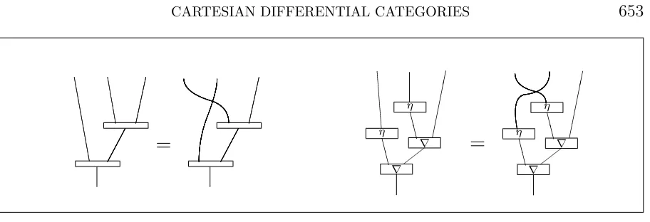
3.2.3. Lemma. In a differential category satisfying the equation 1⊗d⊗;d⊗=c⊗1; 1⊗
d⊗;d⊗, [CD.7] is valid.
Proof. The necessary equation is illustrated in Figure 6.
It will be clear that these proofs are more simply presented using the circuit diagrams; the diagrams for this lemma may be found in Figures 7 and 8. In the diagrams,Ndenotes the Cartesian ∆, and the boxes without half-ovals are Cartesian boxes. Note that we have expanded D×[D×[f]] into a sum, similar to what we did in Figures 4, 5.
The proof of Proposition 3.2.1 then follows from the remark that a differential storage category has the required property, since there d⊗ =η⊗1;∇, and ∇ is cocommutative
and coassociative, as shown in Figure 6.
3.2.4. Remark. We should note here the following property of the coKleisli category
of a differential category with biproducts,viz that ǫand S(f) (for any f) are linear:
• D×[ǫ] = π0ǫ
• D×[S(f)] =π0S(f)
To see the first, recall that ǫ = ǫǫ and π0ǫ = δS(ǫπ0)ǫǫ = ǫπ0ǫ, so D×[ǫ] = s(ǫ⊗
1)D⊗[ǫǫ] =s(ǫ⊗1)(1⊗e)ǫ= ∆(Sπ0⊗Sπ1)(ǫ⊗e)ǫ= ∆(Sπ0⊗e)ǫǫ=Sπ0ǫǫ=ǫπ0ǫ=π0ǫ.
To see the second, recall that S(f) = ǫδS(f), so D×[S(f)] = ∆(Sπ0 ⊗Sπ1)(ǫ⊗
1)D⊗[ǫδS(f)] = ∆(Sπ0⊗Sπ1)(ǫ⊗e)δS(f) = ǫπ0δS(f) =δS(ǫπ0)ǫδS(f) =π0S(f).
These equations are central in arriving at an abstract characterization of coKleisli categories of differential categories, the subject of a sequel to this paper.
4. A term calculus for Cartesian differential categories
f
f
∆
∆
∆
π0
π0 π0
π0 π0
ǫ
ǫ ǫ
ǫ ǫ
π0
π0 π1
π1
π1
✄
✄
+
0 g h k
N N
N
=
Given a map f:X //Y;x7→t, we shall denote the map D×[f]:X×X //Y by the
∂x binds occurrences of x in any operator to which it is applied. So in particular in ∂t
∂x, all occurrences ofx int are bounded. The intention is that ∂t
∂x(s) should determine a linear transformation, so that in a higher-order system it would be typed as
∂t
∂x(s):X −◦Y. In a first-order system we have to use the uncurried form, and so insist that the argument to which it is applied be specified, thus obtaining the term ∂t
∂x(s)·u:Y of type Y; this term is assumed to be linear in u. Of course, we think of this as the x-differential of f, evaluated at x = s. In an “Euler-style” notation, this might be represented by a term like D[x 7→ t](s)·u. The usual “Leibniz-style” notation is something like ∂t
∂x x:=s. Remember our convention is that D×[f] is linear in its first variable, by [CD.2], which
we have been denoting u here. We denote the function application in this case by “·” (as in “dot product”); in the standard example (“high-school differentiation”) it is in fact matrix multiplication.
i.e. by the Jacobian evaluated at (r, s, t). We apply this Jacobian to a vector to obtain a point in IR2:
To summarize: this is what we would write in our term logic as ∂(x2+xyz, z3−xy)
∂(x, y, z) (r, s, t)·(u, v, w)
(compare this to the categorical notation, D×[f]:IR3 ×IR3 //IR2 which takes the pair
((u, v, w),(r, s, t)) to ((2r+st)u+rtv+rsw,−su−rv+ 3t2w)). To help keep in mind
which variables are which, remember that this is supposed to be linear in (u, v, w) (the first variable), not necessarily in the second (r, s, t). Of course, a “variable” may be in fact a tuple of variables, since we are in a Cartesian category.
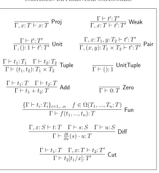
4.1. Definition of the term calculus. Explicit term formation rules for the
Γ, x:T ⊢x:T Proj
Γ⊢t′:T′
Γ, x:T ⊢t′:T′ Weak
Γ⊢t′:T′
Γ,(): 1 ⊢t′:T′ Unit
Γ, x:T1, y:T2 ⊢t′:T′
Γ,(x, y):T1×T2 ⊢t′:T′ Pair
Γ⊢t1:T1 Γ⊢t2:T2
Γ⊢(t1, t2):T1×T2
Tuple
Γ⊢(): 1 UnitTuple Γ⊢t1:T Γ⊢t2:T
Γ⊢t1+t2:T Add Γ⊢0:T Zero
{Γ⊢ti:Ti}i=1,..,n f ∈Ω(T1, ..., Tn;T)
Γ⊢f(t1, ..., tn):T
Fun
Γ, x:S⊢t:T Γ⊢s:S Γ⊢u:S Γ⊢ ∂x∂t(s)·u:T Diff Γ⊢t1:T Γ, x:T ⊢t2:T′
Γ⊢t2[t1/x]:T′
Cut
Table 1: Terms for Cartesian differential logic
a type inT∗×T, we write f ∈Ω(T
1, ..., Tn;T) to indicate a primitive function symbol of
type ([T1, ..., Tn], T). Here we assume that a context Γ consists of a bag of pattern type pairs. The patterns are created by pairing variables or the unit pattern. In a variable context it is always assumed no variable can occurs more than once (i.e. it is linear).
We shall feel free to use n-fold products: these should be interpreted as being con-structed from the binary product using X1×X2×...×Xn= (. . .(X1×X2)×. . .)×Xn
where the association is to the left. The differential operator ∂t
∂x binds the variable x in t; we assume the usual rules on bound and free variables, which in general means it is best not to use the same variable both freely and bound in the same term, and to change bound variables as necessary to maintain that distinction.
The addition is assumed to be a commutative, associative operation with unit 0. Each type therefore contains a 0 and for the final type we have 0: 1 = (): 1
4.1.1. Substitution. The notion t[t′/x] is an explicit substitution term. These terms
[Subst.2] t[(t1, t2)/(p1, p2)]⇒(t[t1/p1])[t2/p2] andt[()/()]⇒t;
4.1.2. Equations of terms. There is an equality defined on the differential term
logic, given by the smallest congruence satisfying the following identities.
[Dt.1] ∂(t1+t2)
(This is the chain rule; we require that no variable of p occur in t);
[Dt.6] ∂
In all these identities we make the usual assumption that they are valid relative to the variable context consisting of those variables mentioned in the identity.
4.2. Basic properties of the term logic. The following lemma provides some
4.2.1. Lemma.
where after the substitution we use the chain rule and then the additivity of the differential twice.
as t contains no variables from p′. The second observation follows by symmetry.
(iv)
Notice that the differential of a map
X1×...×Xn //Y1×...×Ym; (x1, ..., xn)7→(t1, .., tm) can be simplified into the form:
∂(t1, ..., tm)
If we were in a higher order setting we could rewrite this as a matrix calculation:
where a tuple is interpreted as a column vector. This gives the Jacobi form of the differ-ential in terms of the partial derivatives.
Our aim is now to prove the soundness and completeness of this term logic. To prove soundness we must translate the terms into the categorical maps and show that all the equalities hold. To establish completeness we shall build a classifying category for a differential theory.
4.3. Soundness. A differential theory consists of some typesA, some function symbols
Ω, and some equations E between terms of the same type in the same variable context. An interpretation of a differential theory into a Cartesian differential category consists of an assignment of the types in A to objects, M:A //ObjX of the function symbols f ∈ Ω(X1, ..., Xn;X) to maps M(f):M(X1)× ...× M(Xn) // M(X), so that under
the extension of the interpretation to all terms, as defined below, all equations in E are satisfied.
[TC.7] hhp⊢ ∂t
The remainder of this section is given to the proof of the following proposition.
4.3.1. Proposition. The interpretation of terms into a Cartesian differential category
is sound.
The translation of the Cartesian terms is standard. We shall therefore concentrate on the soundness of the translation of the differential terms. To establish the soundness we need to check the identities [Dt.1-7].
[Dt.2]
p⊢ ∂t
∂p′(s)·(u1+u2)
= hh[[p⊢u1+u2]],0i,h[[p⊢s]],1iiD×[[[(p′, p)⊢t]]]
= hh[[p⊢u1]] + [[p⊢u2]],0i,h[[p⊢s]],1iiD×[[[(p′, p)⊢t]]]
= hh[[p⊢u1]],0i+h[[p⊢u2]],0i,h[[p⊢s]],1iiD×[[[(p′, p)⊢t]]]
= hh[[p⊢u1]],0i,h[[p⊢s]],1iiD×[[[(p′, p)⊢t]]]
+hh[[p⊢u2]],0i,h[[p⊢s]],1iiD×[[[(p′, p)⊢t]]]
=
p⊢ ∂t
∂p′(s)·u1+
∂t
∂p′(s)·u2
p⊢ ∂t
∂p′(s)·0
= hh[[p⊢0]],0i,h[[p⊢s]],1iiD×[[[(p′, p)⊢t]]]
= hh0,0i,h[[p⊢s]],1iiD×[[[(p′, p)⊢t]]]
= h0,h[[p⊢s]],1iiD×[[[(p′, p)⊢t]]]
= 0
[Dt.3]
p⊢ ∂x
∂x(s)·u
= hh[[p⊢u]],0i,h[[p⊢s]],1iiD×[[[(x, p)⊢x]]]
= hh[[p⊢u]],0i,h[[p⊢s]],1iiD×[π0]
= hh[[p⊢u]],0i,h[[p⊢s]],1iiπ0π0]
[Dt.4]
[Dt.5] For the chain rule no variable ofp can occur in t:
[Dt.6]
""
q⊢ ∂
∂t ∂p(s)·p
′
∂p′ (s)·u
##
= hh[[q ⊢u]],0i,h[[q⊢s]],1iiD×[
(p′, q)⊢ ∂t
∂p(s)·p
′
]
= hh[[q ⊢u]],0i,h[[q⊢s]],1iiD×[hh[[(p′, q)⊢p′]],0i,h[[(p′, q)⊢s]],1iiD×[[[(p,(p′, q))⊢t]]]]
= hh[[q ⊢u]],0i,h[[q⊢s]],1iiD×[hhπ0,0i,h[[(p′, q)⊢s]],1ii((1×π1)×(1×π1))D×[[[(p, q)⊢t]]]]
= hh[[q ⊢u]],0i,h[[q⊢s]],1iiD×[hhπ0,0i,hπ1[[q⊢s]], π1iiD×[[[(p, q)⊢t]]]]
= hh[[q ⊢u]],0i,h[[q⊢s]],1iihhhπ0π0,0i,h(π1×π1)D×[[[q⊢s]]], π0π1ii,
π1hhπ0,0i,hπ1[[q ⊢s]], π1iiiD×[D×[[[(p, q)⊢t]]]]
= hhh[[q ⊢u]],0i,hh0,1iD×[[[q⊢s]]],0ii,hh[[q ⊢s]],0i,h[[q ⊢s]],1iiiD×[D×[[[(p, q)⊢t]]]]
= hhh[[q ⊢u]],0i,0i,hh[[q ⊢s]],0i,h[[q⊢s]],1iiiD×[D×[[[(p, q)⊢t]]]]
= hh[[q ⊢u]],0i,hh[[q⊢s]],0i,h[[q ⊢s]],1iii(h1,0i ×1)D×[D×[[[(p, q)⊢t]]]]
= hh[[q ⊢u]],0i,hh[[q⊢s]],0i,h[[q ⊢s]],1iii(1×π1)D×[[[(p, q)⊢t]]]
= hh[[q ⊢u]],0i,h[[q⊢s]],1iiD×[[[(p, q)⊢t]]]
=
q ⊢ ∂t
∂p(s)·u
[Dt.7]
where the second-last equation uses the fact that if f is linear (as all projections and pairings of linears are), then D×[f g] = (f ×f)D×[g], and so D×[D×[f g]] =
(f×f ×f×f)D×[D×[g]].
4.4. Completeness. For completeness we form the classifying Cartesian differential
category of a theory. In general here we can permit arbitrary equations. A mapT1 //T2
in the classifying category corresponds to a sequent with one type on the left hand side: p:T1 ⊢t:T2
or evenp7→t when the types may be inferred from the context. Objects: Products of primitive types.
Maps: p7→t:T1 //T2 as above up to provable equality;
Composition: Uses substitution: (p7→t)(p′ 7→t′) = p7→t′[t/p′];
Differential: D×[p7→t:X //Y] = (p′, p)7→ ∂p∂t(p)·p′:X×X //Y.
It is now straightforward to verify that this is a Cartesian differential category. That it is a category is clear, so we only need to verify the axioms [CD.1-7]. [CD.1,2] are obvious.
[CD.3]: D×[1] =π0 follows from
D×[x7→x] = (x′, x)7→
∂x ∂x(x)·x
′
= (x′, x)7→x′ = π
0
D×[π1] =π0π1 follows from
D×[(x, y)7→y] = ((x′, y′),(x, y))7→
∂y
∂(x, y)(x, y)·(x
′, y′)
= ((x′, y′),(x, y))7→ ∂y
∂(x, y)(x, y)·(x
′,0) + ∂y
∂(x, y)(x, y)·(0, y
′)
= ((x′, y′),(x, y))7→ ∂y
∂x(x)·x
′+ ∂y
∂y(y)·y
′
= ((x′, y′),(x, y))7→0 +y′ = y′ = π0π1
(and D×[π0] =π0π0 similarly).
[CD.4]:
D×[hf, gi] = D×[p7→(f, g)]
= (p′, p)7→ ∂(f, g)
∂p (p)·p
′
= (p′, p)7→
∂f ∂p(p)·p
′,∂g
∂p(p)·p
′
![Figure 1: [CD.5] in XS, continued in Figure 2](https://thumb-ap.123doks.com/thumbv2/123dok/924079.902872/28.612.76.534.102.685/figure-cd-in-xs-continued-in-figure.webp)
![Figure 2: [CD.5] in XS, continued from Figure 1](https://thumb-ap.123doks.com/thumbv2/123dok/924079.902872/29.612.76.526.88.689/figure-cd-in-xs-continued-from-figure.webp)
![Figure 3: (1 × π)D×[f] in X](https://thumb-ap.123doks.com/thumbv2/123dok/924079.902872/30.612.73.529.322.644/figure-p-d-f-in-x.webp)
![Figure 5: (⟨1, 0⟩ × 1)D×[D×[f]] in X](https://thumb-ap.123doks.com/thumbv2/123dok/924079.902872/31.612.77.525.211.576/figure-d-d-f-in-x.webp)
![Figure 7: ⟨⟨0, h⟩, ⟨g, k⟩⟩D×[D×[f]]](https://thumb-ap.123doks.com/thumbv2/123dok/924079.902872/33.612.72.526.160.623/figure-h-g-k-d-d-f.webp)
![Figure 8: ⟨⟨0, g⟩, ⟨h, k⟩⟩D×[D×[f]]](https://thumb-ap.123doks.com/thumbv2/123dok/924079.902872/34.612.73.529.246.528/figure-g-h-k-d-d-f.webp)