Mathematics and Informatics ICTAMI 2005 - Alba Iulia, Romania
CONTROL LAWS FREE OF SMOOTH PERTURBATION TERMS
Sorin Stefan Radnef
Abstract. This paper deals with the problem of robust control, from the theory and practical design of control systems, using a general view point which refers only the differential model of controlled object and regarding the reference variable’s trajectory as restrictions for ordinary differential equa-tions, that is as particular integrals (singular solutions). Based on a necessary and sufficient condition to be particular integrals, the restrictions are used to provide the differential model for control laws. This method may reject the perturbation terms that are accurate represented by a power series, at lest on a finite sequence of intervals that cover the entire necessary time domain. A particular case, that serves as an example, is that of an electrohydraulic ser-voactuator designed for reference position tracking. The method generates a structural stable control law which is robust to any modification or perturba-tion of the theoretical model considered.
2000 Mathematics Subject Classification: 93C10, 93C73, 93C95, 93D09. Notations:
x - state variable vector of dimn, in Rn
u - control variable vector of dimn, in U ⊂Rn
λ - constitutive parameters vector of dimp, in Λ ⊂Rp y - output variable vector of dimn
Q reference function - function Q of x and/or y besides of u, that express characteristic properties of system evolution
Q reference trajectory - function R of the independent variable, s, which gives the values of Q
Feasible Q reference trajectory - function R that is possible to be main-tained using adequate control variable law, ur
Control modelling function - vectorial function,g, ofxandu,Im(g)⊂Rm, giving ˙u
Constitutive modelling function - vectorial function,λ, ofxandu,Im(λ)⊂ Rp
Output modelling function - vectorial function,h, ofxandu,Im(h)⊂Rn, giving y
Restriction function - implicit function,W, defined asW(x, u, s)≡Q(x, u)− R(s)
Restriction equation - equation derived considering W as well defining a singular solution of the differential system for ˙x and ˙u
Reference state and control variable, xr, ur - state and control variable corresponding to the feasible Qreference trajectory
Introduction and statement of the general problem
The origin of this paper is the thought to treat in a unified manner and to solve using a unique conceptual procedure almost all the control problems. First attempt was made in [5], and developed in [4]. To show the method and its significant results it is useful to approach a less difficult problem, as is the one of the reference [1], regarding the state-tracking problem for an electro-hydraulic servo, solved there using a neuro-fuzzy controller, that is solved by an extrinsic procedure. In a preceding paper of the authors, [2], the problem was solved by an intrinsic procedure, but having a definite specific and a little cumbersome character.
A coherent and consistent treatment of the control problem, in a unified manner using a single view point, as an inverse problem, is the reference [3]. The papers [5], [6], [7], [8] and the thesis [4] follow this view point and develops an algorithmic procedure to solve the control problem as an inverse problem, in fact to solve the differential algebraic (system of) equation(s) that represent the evolution of a controlled physical object.
So, the self consistent model (that is autonomous) of state-feedback control problem becomes:
˙
x=f(x, u;λ) ˙
u=g(x, u;λ) (1)
Q(x, u) =R(s) (2)
considering s a monotonous function of time variable or, for output-feedback control problem:
˙
x=f(x, u;λ) ˙
u=g(y, u;λ)
y =h(x, u;λ)
(3)
Q(y, u) =R(s) (4)
This way, the three well known types of control problems are defined by means of Q reference trajectory properties:
(a) stability with respect to Q reference function trajectory of a defined evolution of (1)
(b) optimality regarding extreme/ limiting values ofQreference trajectory (c) tracking a predefined Q reference trajectory.
In fact we have two problems to solve:
(1) statement the values of the Q reference function (2) tracking the Q reference function
after we have had solved the construction of an adequate Qreference func-tion for the objective we have to achieve. The first condifunc-tion for the (1) or (3) control problem is to be a well posed problem, which isQreference function be a feasible one. The first problem, which may include the optimality one by a set of mathematical restrictions, is considered for the purpose of this paper as solved and we treat only the second one, which may be formulated as follows:
”Giving the differential model of the physical system evolution ˙
x=f(x, u;λ) ˙
u=g(x, u;λ)
lim t→∞
||Q(x, u)−R(s)||= 0”
The solution of the so formulated state-tracking problem is approached regarding the restriction function defined by the implicit equation:
Q(x, u)−R(s) = 0 (5)
and denoted by W(σ, u) with σ = (x, l)T, as a singular integral of the dif-ferential system (1). The necessary and sufficient condition for (5) to be a sin-gular integral of (1) provide, following the results of [4] and [8], the restriction equation which determine the control modeling function g. The algorithmic procedure developed in [4] and [8] ensures a step by step construction of the appropriate restriction equation for g function establishment.
A brief presentation of the results of [4], [8], that will be used throughout if this paper, is quite necessary to understand the method to determine as solution of the control problem. The main fact is that of the following lemma: Lemma NSC. The necessary and sufficient condition that the algebraic equation:
0 = W(σ, u)
may determine a singular solution of (1) system is:
W(σ, u) = 0 =⇒0 = Wσ ·f(σ, u) +Wu·g(σ, u) So, we take into account that:
(1) Between the values of Wσ ·f(σ, u) +Wu·g(σ, u) and the values w of
W(·) seems to be a relationship which is of function type for w= 0
(2) For each value w of W(·) we choose a single value of u to reach the zero value of W(·) in an asymptotic way (at least),
and by consequence, we are able to define the following function: Φ :Im(W)×Dom(W)→Rq,
having the values for(w, σ, u)∈Im(W)×Dom(W)defined by the analytical formula:
with the following features:
(σ, u)∈R2 →(0≡Φ(0, σ, u)and06= Φ(w6= 0, σ, u)) (7)
Φ∈C−1
(Im(W)×Dom(W), Rq) (8)
This way, the necessary and sufficient condition (NSC) is expressed by the relation (RE), with (7), (8) defining features, supposing that it has solutions on Dom(W). The Φ function is a fitting indicator for W to be a singular implicit solution of (1) and represent the time rate of W along the regular solutions of (1).
DW
Dt 1 = Φ(W, σ, u) (9)
Hence one can prescribe the structure of this function and thus defining the dynamics of nonzero values of W . Tacking into account these meanings, the Φ function may be named “perturbation function”. The basic requirement for the perturbation function is to provide a stable and (uniform) asymptotic behavior of W around the zero value, that is we may find at least one δ0 ∈R+
so that:
((σ0, u0),||W(σ0, u0)||< δ0)→ lim t→∞
W(σ(t, σ0, u0), u(t, σ0, u0))|(DS) = 0 (10)
As a particular situation, Φ may have a linear structure like this: Φ(w, σ, u)≡Φ(W) = S·W
with S a stability matrix for the differential system with respect toW: ˙
W =S·W (11)
(RE) Corollary.The (6) relation with perturbation function having the properties (7), (8), (10) is the necessary and sufficient condition for the re-striction function to define a singular implicit solution of (1).
To simplify the style statement of ”(RE) Corollary” we denote (12) the set {(6), (7), (8), (10)}. So, the necessary and sufficient condition for the restriction function to be a singular implicit solution is (12). The differential modeling function for control variables,g, derives from the restriction equation:
Wσ·f(σ, u) +Wu·g(σ, u) = Φ(W, σ, u)∼=S·W (12) If rank(Wu) = m , (12) determines the differential modeling function U . Whenrank(Wu) = q < mit is necessary to find out a new adequate restriction function following the same requirements and rules used to obtain (6). Because (12) is, in fact the essential necessary and sufficient condition upon W to be singular implicit solution for (1), it becomes in a very natural way the new restriction function to continue the algorithm for finding all the components of g function. So:
0 = Wσ ·f(σ, u) +Wu ·g(σ, u)−Φ(W, σ, u)∼= ˜W(W, σ, u, U) (13) and not Wσ · f(σ, u) +Wu ·g(σ, u) ≡ W˜(σ, u) as is the usual procedure in [3]. This way there are preserved the intrinsic characteristics of (6) and the stability of W function. Also (13) provide an algorithm to determine the differential modeling function for all control variables, at each step using the fundamental lemma NSC for a new inverse problem. The coherent formulation for the preceding explanations is the
Recurrence theorem. If W is the current restriction function, and is the new one defined by (13) with Φ the current perturbation function.
Then (12) constructed for W˜ maintain the (12) for W with its stable and asymptotic behavior around zero value.
Nonlinear System Control to be Solved
The differential model of the electrohydraulic servo is, [1], [2]: ˙
x1 =x2
˙
x2 =a1x1+a2x2+Kup+p(t, x)
˙
x3 =B{cwkvs|u|sgn[pa(1+sgn(kvsu))−2x3] r
|pa(1 +sgn(kvsu))−2x3|
ρ −Sx2
C−Sx1
˙
x4 =B{cwkvs|u|sgn[pa(1−sgn(kvsu))−2x4] r
|pa(1 +sgn(kvsu))−2x4|
ρ −Sx2
C−Sx1
having the control variables up = x3−x4, the overall acting pressure on the piston, and u the electrical control quantity, and p(t, .) as the “forcing function”. The constitutive parameters are:
λ = [a1a2K B c w kvspaρ S C]T
with values from [1], [2]. The Qreference function isQp(x, u) =x1 and the feasible Q reference trajectoryR(t) = x1s(1−e−1
tr).
This state-tracking problem is solved by splitting the differential model in two subsystems:
˙
x1 =x2
˙
x2 =a1x1+a2x2+Kup+p(t, x)
that describe the dynamic behavior of the principal mechanical device which must be controlled by up , having the Q reference function just men-tioned above, and
˙
x3 =B{cwkvs|u|sgn[pa(1+sgn(kvsu))−2x3] r
|pa(1 +sgn(kvsu))−2x3|
ρ −Sx2
C−Sx1
˙
x4 =B{cwkvs|u|sgn[pa(1−sgn(kvsu))−2x4]
r
|pa(1 +sgn(kvsu))−2x4|
ρ −Sx2
C−Sx1
that describes the dynamic behavior of the hydraulic device which controls the principal mechanical device, having u the control variable, theQreference function Qc(x, u) = x3−x4 and the feasible Q reference trajectoryR(t) =up.
necessary values of the variableup. These values will be the reference trajectory to solve the second control problem.
The method to solve each of these two control systems, with its own refer-ences, is that presented in the former chapter.
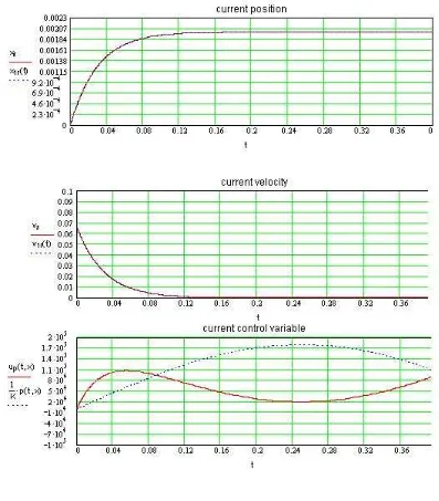
Position Tracking for a Servoactuator
For the dynamics of the first subsystem, the restriction equation will be find using the linear structure of the perturbation function. Performing two steps of the algorithm presented at the first chapter, we derive:
¨
x1−x¨1r−(λ1+λ2)·( ˙x1+ ˙x2r) + (λ1·λ2)·(x1+x1r) = 0
having λk=1,2 negative real values, and then:
up = 1
K[−a1x1−a2x2−p(t, x)+(λ1+λ2)·(x1−x1˙ r)−(λ1λ2)·(x1+x1r)+¨x1r] (14)
where we have denoted by x1r the reference variable provided by the Q reference trajectory functionR.
The elements of the feasible Qreference trajectory are in Figure 1.
The tracking relative error is smaller than 10−4 .
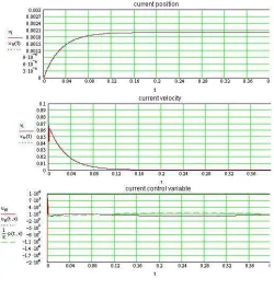
It is possible to arrive at a higher order restriction equation by building successively new restriction function of the type (13). Aftern steps we derive the restriction equation:
0 = n X
k=0
Sk(x(n−k)
1 −x (n−k)
1r ) (15)
having Sk as the sum of products build with k negative real numbers
Figure 2:
¨
up = 1
K[−a1x2˙ +x (4)
1r+S1(x
(2) 2 −x
(3)
1r)−S3(x
(1) 2 −x
(2)
1r)+S3(x2−x
(1)
1r)−S4(x1−x1r)] (16) The forcing function does not appear explicitly in the above formula, but its existence and effects are contained in the values of the state variables x1,2
and their time derivatives. Using this kind of control modelling function we have obtained the elements of the feasible Q reference trajectory as those presented in the following diagrams (Figure 2), considering also some starting perturbations.
The tracking relative error is smaller than 10−4 .
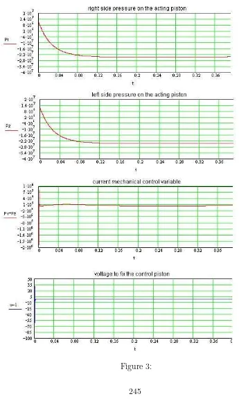
For the dynamics of the second subsystem, the control one, the results concerning the state variables, x3 :=p1 and x4 := p2, and control variable u
[image:10.612.171.421.91.356.2]Conclusions
The procedure proposed in this paper allows:
1) quickly solutions for the analysis of the nonlinear control problem (feasible Q reference trajectory, influence of initial perturbations, . . . )
2) a complete ignoring of forcing function, that is a robust (and stable) control
3) the split of a (very) difficult (tracking) control problem into more easy to solve control problems
It must be underlined that even the system ˙x = f(x, u;λ) is stable for everyuas parameters the extended system (1) may be unstable. Therefore the negative numbersλused in the control modelling function must be determined according to the relations which define the stability behavior of the differential system (1), as is specified explicitly in [8].
References
[1] Ioan Ursu, Felicia Ursu, Lucian Iorga, Neuro-fuzzy Synthesis of Flight Control Electrohydraulic Servo, Aircraft Engineering andAerospace Technol-ogy, MCB University Press, vol. 73, no. 5, 2001
[2] Ioan Ursu, George Tecuceanu, Felicia Ursu, Mihai Vladimirescu, From Robust Control to Antiwindup Compensation of Electrohydraulic servo Actua-tors, Aircraft Engineering and Aerospace Technology, MCB University Press, vol. 70, no. 4, 1998
[3] Galiulin, A. S.,Inverse Problems of Dynamics, Mir Publishers, Moscow, 1984
[4] Sorin Stefan Radnef, Studies Concerning Flight Dynamics and Con-trol in Pursuit/ Tracking Problems, Ph D Thesis, Polytechnic University of Bucharest, AeroSpace Sciences Department, Mach 15 2002, Bucharest
[5] Sorin Stefan Radnef, Dynamic Model for the Controlled Motion along a Given Flight Path, paper 3485-95 presented at AIAA Atmospheric Flight Mechanics Conference, Baltimore, Aug. 7-9, 1995, USA.
[6] Sorin Stefan Radnef, A General Inverse Problem in Controlled Flight Movement, paper presented at SACAM ’96, Eskom, Midrand Gauteng, South Africa, proceedings vol. 2.
[8] Sorin Stefan Radnef,Differential Modelling of DAEs Solutions for Flight Control, paper presented at ICNPAA 2004, June 02-04.2004, West Univer-sity, Timisoara, Romania, proceedings of the 5th, International Conference on Mathematical Problems in Engineering and Aerospace Sciences, Cambridge Scientific Publishers ltd., UK
[9] Baumgarte J., Stabilization of Constraints and Integrals of Motion in Dynamical wSystems, Computer Methods in Applied Mechanics and Engineer-ing, 1, 1972
Sorin Radnef
National Institute of AeroSpatial Research, Flight Dynamics Department Romania