getdocc076. 375KB Jun 04 2011 12:04:55 AM

El e c t ro n ic

Jo ur

n a l o

f P

r o

b a b i_{l i t y}

Vol. 15 (2010), Paper no. 48, pages 1487–1527. Journal URL

http://www.math.washington.edu/~ejpecp/

Multi-dimensional Gaussian fluctuations

on the Poisson space

Giovanni Peccati

∗

Cengbo Zheng

†

Abstract

We study multi-dimensional normal approximations on the Poisson space by means of Malli-avin calculus, Stein’s method and probabilistic interpolations. Our results yield new multi-dimensional central limit theorems for multiple integrals with respect to Poisson measures – thus significantly extending previous works by Peccati, Solé, Taqqu and Utzet. Several explicit exam-ples (including in particular vectors of linear and non-linear functionals of Ornstein-Uhlenbeck Lévy processes) are discussed in detail.

Key words: Central Limit Theorems; Malliavin calculus; Multi-dimensional normal approxi-mations; Ornstein-Uhlenbeck processes; Poisson measures; Probabilistic Interpolations; Stein’s method.

AMS 2000 Subject Classification:Primary 60F05; 60G51; 60G57; 60H05; 60H07. Submitted to EJP on April 10, 2010, final version accepted August 16, 2010.

∗_{Faculté des Sciences, de la Technologie et de la Communication; UR en Mathématiques. 6, rue Richard} Coudenhove-Kalergi, L-1359 Luxembourg. Email:giovanni.peccati@gmail.com

†_{Equipe Modal’X, Université Paris Ouest – Nanterre la Défense, 200 Avenue de la République, 92000 Nanterre, and}

1

Introduction

Let(Z,_Z,µ)be a measure space such that Z is a Borel space andµis aσ-finite non-atomic Borel measure. We setZµ = {B ∈ Z :µ(B)<∞}. In what follows, we write Nˆ ={Nˆ(B): B ∈ Zµ}to

indicate acompensated Poisson measureon(Z,_Z)withcontrolµ. In other words,Nˆ is a collection of random variables defined on some probability space (Ω,_F,P), indexed by the elements of _Zµ and such that: (i) for every B,C ∈ Zµ such thatB∩C =∅, the random variablesNˆ(B) andNˆ(C)

are independent; (ii) for every B _{∈ Zµ}, Nˆ(B)(l aw=)N(B)₋µ(B), where N(B)is a Poisson random variable with paremeter µ(B). A random measure verifying property (i) is customarily called “completely random” or, equivalently, “independently scattered” (see e.g. [25]).

Now fixd_≥2, let F= (F₁, . . . ,F_d)_⊂ L2(σ( ˆN),P)be a vector of square-integrable functionals ofNˆ, and letX = (X1, . . . ,Xd)be a centered Gaussian vector. The aim of this paper is to develop several

techniques, allowing to assess quantities of the type

d_H(F,X) = sup

g∈H|

E[g(F)]₋E[g(X)]_|, (1)

where _H is a suitable class of real-valued test functions onRd. As discussed below, our principal aim is the derivation of explicit upper bounds in multi-dimensional Central limit theorems (CLTs) involving vectors of general functionals of Nˆ. Our techniques rely on a powerful combination of Malliavin calculus (in a form close to Nualart and Vives [15]), Stein’s method for multivariate normal approximations (see e.g. [5, 11, 23]and the references therein), as well as some interpo-lation techniques reminiscent of Talagrand’s “smart path method” (see[26], and also[4, 10]). As such, our findings can be seen as substantial extensions of the results and techniques developed e.g. in [9, 11, 17], where Stein’s method for normal approximation is successfully combined with infinite-dimensional stochastic analytic procedures (in particular, with infinite-dimensional integration by parts formulae).

The main findings of the present paper are the following:

(I) We shall use both Stein’s method and interpolation procedures in order to obtain explicit upper bounds for distances such as (1). Our bounds will involve Malliavin derivatives and infinite-dimensional Ornstein-Uhlenbeck operators. A careful use of interpolation techniques also allows to consider Gaussian vectors with a non-positive definite covariance matrix. As seen below, our estimates are the exact Poisson counterpart of the bounds deduced in a Gaussian framework in Nourdin, Peccati and Réveillac[11]and Nourdin, Peccati and Reinert[10].

(II)The results at point(I)are applied in order to derive explicit sufficient conditions for multivari-ate CLTs involving vectors of multiple Wiener-Itô integrals with respect toNˆ. These results extend to arbitrary orders of integration and arbitrary dimensions the CLTs deduced by Peccati and Taqqu

[18]in the case of single and double Poisson integrals (note that the techniques developed in[18]

to joint convergence. (See also [11].) As demonstrated in Section 6, this property is particularly useful for applications.

The rest of the paper is organized as follows. In Section 2 we discuss some preliminaries, including basic notions of stochastic analysis on the Poisson space and Stein’s method for multi-dimensional normal approximations. In Section 3, we use Malliavin-Stein techniques to deduce explicit upper bounds for the Gaussian approximation of a vector of functionals of a Poisson measure. In Section 4, we use an interpolation method (close to the one developed in [10]) to deduce some variants of the inequalities of Section 3. Section 5 is devoted to CLTs for vectors of multiple Wiener-Itô integrals. Section 6 focuses on examples, involving in particular functionals of Ornstein-Uhlenbeck Lévy processes. An Appendix (Section 7) provides the precise definitions and main properties of the Malliavin operators that are used throughout the paper.

2

Preliminaries

2.1

Poisson measures

As in the previous section,(Z,Z,µ)is a Borel measure space, andNˆ is a Poisson measure onZ with controlµ.

Remark 2.1. Due to the assumptions on the space(Z,Z,µ), we can always set(Ω,_F,P)andNˆ to be such that

Ω =

  ω=

n

X

j=0

δzj,n∈N∪ {∞},zj∈Z

  

whereδzdenotes the Dirac mass atz, andNˆ is thecompensated canonical mapping

ω7→Nˆ(B)(ω) =ω(B)₋µ(B), B_{∈ Zµ}, ω∈Ω,

(see e.g. [21]for more details). For the rest of the paper, we assume thatΩ andNˆ have this form. Moreover, theσ-field_F is supposed to be theP-completion of theσ-field generated byNˆ.

Throughout the paper, the symbol L2(µ) is shorthand for L2(Z,_Z,µ). For n_≥2, we write L2(µn) and L_s2(µn_{), respectively, to indicate the space of real-valued functions on Z}n _{which are}

square-integrable with respect to the product measureµn, and the subspace of L2(µn)composed of sym-metric functions. Also, we adopt the convention L2(µ) = L_s2(µ) = L2(µ1) = L2_s(µ1) and use the following standard notation: for everyn≥1 and every f,g∈L2(µn_),

〈f,g_〉L2_(µn₎=

Z

Zn

f(z₁, ...,z_n)g(z₁, ...,z_n)µn(dz₁, ...,dz_n), _kf_kL2_(µn₎=〈f,f〉1/2

L2_(µn₎.

For every f ∈L2(µn_{), we denote by} e_{f the canonical symmetrization of f, that is,}

e

f(x₁, . . . ,x_n) = 1

n!

X

σ

whereσruns over then! permutations of the set_{1, . . . ,n_}. Note that, e.g. by Jensen’s inequality,

kf˜_kL2_(µn₎≤ kfk_L2_(µn₎ (2)

For every f _∈L2(µn),n_≥1, and every fixedz_∈Z, we write f(z,_·)to indicate the function defined on Zn−1 given by(z1, . . . ,zn−1)7→ f(z,z1, . . . ,zn−1). Accordingly,âf(z,·) stands for the

symmetriza-tion of the funcsymmetriza-tion f(z,_·)(in(n₋1)variables). Note that, ifn=1, then f(z,_·) = f(z)is a constant.

Definition 2.2. For every deterministic function h_∈ L2(µ), we write I₁(h) = ˆN(h) = R_Zh(z) ˆN(dz)

to indicate the Wiener-Itô integralof h with respect to N . For every nˆ ≥ 2and every f ∈ L_s2(µn_),

we denote by I_n(f)themultiple Wiener-Itô integral, of order n, of f with respect toN . We also setˆ In(f) =In(˜f), for every f ∈L2(µn), and I0(C) =C for every constant C.

The reader is referred e.g. to Peccati and Taqqu[19]or Privault[22]for a complete discussion of multiple Wiener-Itô integrals and their properties (including the forthcoming Proposition 2.3 and Proposition 2.4) – see also[15, 25].

Proposition 2.3. The following properties hold for every n,m_≥1, every f _∈ L_s2(µn) and every g _∈ L_s2(µm_):

1. E[I_n(f)] =0,

2. E[I_n(f)I_m(g)] =n!〈f,g〉L2_(µn₎1_(n=m)(isometric property).

The Hilbert space composed of the random variables with the form I_n(f), where n_≥ 1 and f _∈ L_s2(µn), is called the nthWiener chaos associated with the Poisson measureNˆ. The following well-knownchaotic representation propertyis essential in this paper.

Proposition 2.4 (Chaotic decomposition). Every random variable F ∈ L2(_F,P) = L2(P)admits a (unique) chaotic decomposition of the type

F=E[F] + ∞

X

n≥1

I_n(f_n) (3)

where the series converges in L2(P)and, for each n_≥1, the kernel f_nis an element of L2_s(µn).

2.2

Malliavin operators

For the rest of the paper, we shall use definitions and results related to Malliavin-type operators defined on the space of functionals of the Poisson measure Nˆ. Our formalism is analogous to the one introduced by Nualart and Vives [15]. In particular, we shall denote by D, δ, L and L−1, respectively, the Malliavin derivative, the divergence operator, the Ornstein-Uhlenbeck generator

and its pseudo-inverse. The domains of D, δ and L are written domD, domδ and domL. The domain of L−1 is given by the subclass of L2(P) composed of centered random variables, denoted by L2₀(P).

underlying probability space Ω is assumed to be the collection of discrete measures described in Remark 2.1, then one can meaningfully define the random variableω7→Fz(ω) =F(ω+δz),ω∈Ω,

for every given random variable F and every z ∈ Z, where δ_z is the Dirac mass at z. One can therefore prove that the following neat representation ofDas adifference operatoris in order.

Lemma 2.5. For each F∈domD,

D_zF=F_z−F, a.e.-µ(dz).

A proof of Lemma 2.5 can be found e.g. in [15, 17]. Also, we will often need the forthcoming Lemma 2.6, whose proof can be found in[17](it is a direct consequence of the definitions of the operatorsD,δandL).

Lemma 2.6. One has that F∈domL if and only if F∈domD and DF ∈domδ, and in this case

δDF=₋L F.

Remark 2.7. For every F_∈L2₀(P), it holds that L−1F_∈domL, and consequently

F=L L−1F =δ(₋D L−1F) =₋δ(D L−1F).

2.3

Products of stochastic integrals and star contractions

In order to give a simple description of themultiplication formulaefor multiple Poisson integrals (see formula (6)), we (formally) define a contraction kernel f⋆l_rgonZp+q−r−l for functions f ∈L_s2(µp) andg_∈L_s2(µq), where p,q_≥1,r=1, . . . ,p_∧qandl=1, . . . ,r, as follows:

f ⋆l_rg(γ1, . . . ,γr−l,t1, , . . . ,tp−r,s1, , . . . ,sq−r) (4)

=

Z

Zl

µl(dz₁, ...,dz_l)f(z₁, , . . . ,z_l,γ1, . . . ,γr−l,t1, , . . . ,tp−r)

×g(z₁, , . . . ,z_l,γ1, . . . ,γr−l,s1, , . . . ,sq−r).

In other words, the star operator “⋆l_r” reduces the number of variables in the tensor product of f

andgfromp+qtop+q₋r₋l: this operation is realized by first identifyingr variables in f andg, and then by integrating outl among them. To deal with the casel=0 forr=0, . . . ,p_∧q, we set

f ⋆0_rg(γ1, . . . ,γr,t1, , . . . ,tp−r,s1, , . . . ,sq−r)

= f(γ1, . . . ,γr,t1, , . . . ,tp−r)g(γ1, . . . ,γr,s1, , . . . ,sq−r),

and

f ⋆0₀g(t1, , . . . ,tp,s1, , . . . ,sq) = f ⊗g(t1, , . . . ,tp,s1, , . . . ,sq) = f(t1, , . . . ,tp)g(s1, , . . . ,sq).

By using the Cauchy-Schwarz inequality, one sees immediately that f ⋆r_r g is square-integrable for any choice ofr =0, . . . ,p_∧q, and every f _∈L_s2(µp), g_∈L_s2(µq).

Definition 2.8. Let p_≥1and let f _∈L2_s(µp).

1. If p≥1, the kernel f is said to satisfyAssumption A, if(f⋆pp−rf)∈L2(µr)for every r =1, ...,p.

Note that(f ⋆0_p f)_∈L2(µp)if and only if f _∈L4(µp).

2. The kernel f is said to satisfyAssumption B, if: either p=1, or p_≥2and every contraction of the type

(z1, ...,z2p−r−l)7→ |f|⋆lr|f|(z1, ...,z2p−r−l)

is well-defined and finite for every r = 1, ...,p, every l = 1, ...,r and every (z1, ...,z2p−r−l) ∈

Z2p−r−l.

The following statement will be used in order to deduce the multivariate CLT stated in Theorem 5.8. The proof is left to the reader: it is a consequence of the Cauchy-Schwarz inequality and of the Fubini theorem (in particular, Assumption A is needed in order to implicitly apply a Fubini argument – see step (S4) in the proof of Theorem 4.2 in[17]for an analogous use of this assumption).

Lemma 2.9. Fix integers p,q_≥1, as well as kernels f _∈L_s2(µp)and g_∈L_s2(µq)satisfying Assumption A in Definition 2.8. Then, for any integers s,t satisfying 1_≤ s _≤ t _≤ p_∧q, one has that f ⋆s_t g _∈ L2(µp+q−t−s_{), and moreover}

1.

kf ⋆s_t g_k2_L2_(µp+q−t−s₎=〈f ⋆

p−t p−s f,g⋆

q−t

q−s g〉L2_(µt+s₎, (and, in particular,

kf ⋆s_t fkL2_(µ2p−s−t₎=kf ⋆p_p−_−st fk_L2_(µt+s₎); 2.

kf ⋆s_t gk2_L2_(µp+q−t−s₎ ≤ kf ⋆

p−t

p−s fkL2_(µt+s₎× kg⋆_qq−_−st gk_L2_(µt+s₎

= _kf ⋆s_t f_kL2_(µ2p−s−t₎× kg⋆s

tgkL2_(µ2q−s−t₎.

Remark 2.10. 1. Writing k= p+q−t−s, the requirement that 1≤s≤t ≤p∧qimplies that |q₋p_{| ≤}k_≤p+q₋2.

2. One should also note that, for every 1_≤p_≤qand every r=1, ...,p,

Z

Zp+q−r

(f ⋆0_rg)2dµp+q−r=

Z

Zr

(f ⋆p_p−r f)(g⋆_qq−rg)dµr, (5)

for every f ∈L2_s(µp_{)and every g∈ L}2

s(µq), not necessarily verifying Assumption A. Observe

that the integral on the RHS of (5) is well-defined, since f ⋆pp−r f ≥0 andg⋆ q−r q g≥0.

3. Fix p,q _≥ 1, and assume again that f _∈ L2_s(µp) and g _∈ L2_s(µq) satisfy Assumption A in Definition 2.8. Then, a consequence of Lemma 2.9 is that, for everyr =0, ...,p∧q−1 and everyl=0, ...,r, the kernel f(z,_·)⋆l_rg(z,_·)is an element of L2(µp+q−t−s−2)forµ(dz)-almost everyz_∈Z.

Proposition 2.11(Product formula). Let f _∈L_s2(µp)and g_∈L_s2(µq), p,q_≥1, and suppose moreover that f ⋆l_r g∈L2(µp+q−r−l)for every r=1, . . . ,p∧q and l=1, . . . ,r such that l6=r. Then,

I_p(f)I_q(g) =

p∧q

X

r=0

r!

‚

p r

Œ ‚

q r

Œ_Xr

l=0 ‚

r l

Œ

I_p+q−r−l

 â_{f ⋆}l

rg

‹

, (6)

with the tilde∼indicating a symmetrization, that is,

â_{f ⋆}l

r g(x1, . . . ,xp+q−r−l) =

1

(p+q−r−l)!

X

σ

f ⋆l_rg(x_σ(1), . . . ,x_{σ(p+q−r−l)}),

whereσruns over all(p+q₋r₋l)!permutations of the set_{1, . . . ,p+q₋r₋l_}.

2.4

Stein’s method: measuring the distance between random vectors

We write g ∈Ck(Rd) if the function g : Rd _→ R admits continuous partial derivatives up to the orderk.

Definition 2.12. 1. TheHilbert-Schmidt inner productand theHilbert - Schmidt normon the class of d_×d real matrices, denoted respectively by_〈·,_·〉H.S.and_{k · kH.S.}, are defined as follows: for every pair of matrices A and B,〈A,B〉H.S.:=T r(ABT)andkAkH.S.=

p

〈A,A〉H.S., where T r(·)

indicates the usual trace operator.

2. Theoperator normof a d×d real matrix A is given bykAkop:=sup_kxkRd=1kAxkR

d.

3. For every function g:Rd_7→R, let

kgkLi p:=sup x6=y

|g(x)₋g(y)_| kx₋y_kRd

,

where_{k · k}Rd is the usual Euclidian norm onRd. If g∈C1(Rd), we also write

M₂(g):=sup

x6=y

k∇g(x)_{− ∇}g(y)_kRd

kx₋ y_kRd

,

If g∈C2(Rd),

M3(g):=sup

x6=y

kHessg(x)₋Hessg(y)_kop kx₋ y_kRd

,

whereHessg(z)stands for the Hessian matrix of g evaluated at a point z.

4. For a positive integer k and a function g∈Ck(Rd), we set

kg(k)_k∞= max

1≤i1≤...≤ik≤d

sup

x∈Rd

∂k ∂xi1. . .∂xik

g(x)

In particular, by specializing this definition to g(2)=g′′and g(3)=g′′′, we obtain

kg′′k∞=₁ max ≤i1≤i2≤d_xsup_∈Rd

∂2 ∂x_i

1∂xi2

g(x)

.

kg′′′k∞=₁ max

≤i1≤i2≤i3≤d_xsup_∈Rd

∂3 ∂x_i

1∂xi2∂xi3

g(x)

.

Remark 2.13. 1. The normkgkLi p is writtenM1(g)in[5].

2. Ifg∈C1(Rd), then_kgkLi p= sup x∈Rd

k∇g(x)_kRd. Ifg∈C2(Rd), then

M₂(g) = sup

x∈Rd

kHessg(x)_kop.

Definition 2.14. The distance d₂ between the laws of two Rd-valued random vectors X and Y such thatE_kX_kRd,EkYk_Rd <∞, written d₂(X,Y), is given by

d2(X,Y) = sup

g∈H|

E[g(X)]₋E[g(Y)]_|,

where_H indicates the collection of all functions g_∈C2(Rd)such that_kg_{kLi p≤}1and M₂(g)_≤1.

Definition 2.15. The distance d3 between the laws of two Rd-valued random vectors X and Y such

thatE_kX_k2_Rd,EkYk

2

Rd <∞, written d3(X,Y), is given by

d3(X,Y) = sup

g∈H|

E[g(X)]₋E[g(Y)]_|,

whereH indicates the collection of all functions g∈C3(Rd)such thatkg′′k∞≤1andkg′′′k∞≤1. Remark 2.16. The distancesd2 andd3 are related, respectively, to the estimates of Section 3 and

Section 4. Let j = 2, 3. It is easily seen that, if d_j(F_n,F)_→ 0, where F_n,F are random vectors in

Rd, then necessarilyF_n converges in distribution toF. It will also become clear later on that, in the definition of d₂ andd₃, the choice of the constant 1 as a bound for_kg_{kLi p},M₂(g),_kg′′_k∞,_kg′′′_k∞

is arbitrary and immaterial for the derivation of our main results (indeed, we definedd2 andd3 in

order to obtain bounds as simple as possible). See the two tables in Section 4.2 for a list of available bounds involving more general test functions.

The following result is a d-dimensional version of Stein’s Lemma; analogous statements can be found in [5, 11, 23] – see also Barbour [1] and Götze [6], in connection with the so-called “generator approach” to Stein’s method. As anticipated, Stein’s Lemma will be used to deduce an explicit bound on the distance d2 between the law of a vector of functionals of Nˆ and the law of

a Gaussian vector. To this end, we need the two estimates (7) (which is proved in [11]) and (8) (which is new).

Lemma 2.17 (Stein’s Lemma and estimates). Fix an integer d _≥ 2 and let C = _{C(i,j) : i,j = 1, . . . ,d}be a d×d nonnegative definite symmetric real matrix.

1. Let Y be a random variable with values inRd_{. Then Y ∼ Nd}(0,C)if and only if, for every twice differentiable function f :Rd _7→R such that E_|〈C, Hessf(Y)_〉H.S.|+E_|〈Y,_∇f(Y)_〉Rd| <∞, it

holds that

E[_〈Y,∇f(Y)_〉Rd− 〈C, Hessf(Y)〉_H.S.] =0

2. Assume in addition that C is positive definite and consider a Gaussian random vector X _∼

Nd(0,C). Let g:Rd7→Rbelong toC2(Rd)with first and second bounded derivatives. Then, the

function U0(g)defined by

U₀g(x):=

Z 1

0

1

2tE[g(

p

t x+p1₋t X)₋g(X)]d t

is a solution to the following partial differential equation (with unknown function f ):

g(x)₋E[g(X)] =_〈x,_∇f(x)_〉Rd− 〈C, Hessf(x)〉_H.S., x ∈Rd.

Moreover, one has that

sup

x∈Rdk

HessU₀g(x)_{kH.S.≤ k}C−1_kopkC_k1_op/2_kg_{kLi p}, (7)

and

M3(U0g)≤

p 2π

4 kC −1

k3op/2kCkopM2(g). (8)

Proof. We shall only show relation (8), as the proof of the remaining points in the statement can be found in[11]. SinceC is a positive definite matrix, there exists a non-singular symmetric matrixA

such thatA2=C, andA−1X ∼ Nd(0,Id). LetU0g(x) =h(A−1x), where

h(x) =

Z 1

0

1

2tE[gA(

p

t x+p1₋tA−1X)₋g_A(A−1X)]d t

andg_A(x) =g(Ax). AsA−1X_{∼ Nd}(0,I_d), the functionhsolves the Stein’s equation 〈x,∇h(x)_〉Rd−∆h(x) =g_A(x)−E[g_A(Y)],

whereY _{∼ Nd}(0,I_d)and∆is the Laplacian. On the one hand, as Hessg_A(x) =AHessg(Ax)A(recall thatAis symmetric), we have

M₂(g_A) = sup

x∈Rdk

Hessg_A(x)_kop= sup

x∈Rdk

AHessg(Ax)A_kop

= sup

x∈Rd

kAHessg(x)Akop≤ kAk2opM2(g)

= _kCkopM2(g),

where the inequality above follows from the well-known relation_kAB_{kop≤ k}A_kopkB_kop. Now write

h_A−1(x) =h(A−1x): it is easily seen that

It follows that

M3(U0g) = M3(hA−1)

= sup

x6=y

kHessh_A−1(x)−Hessh_A−1(y)k_op

kx₋y_k

= sup

x6=y

kA−1Hessh(A−1x)A−1−A−1Hessh(A−1y)A−1kop

kx−yk

≤ kA−1_k2_op×sup

x6=y

kHessh(A−1x)₋Hessh(A−1y)_kop

kx−yk ×

kA−1x₋A−1y_k

kA−1_x−A−1_yk

≤ kA−1k2op×sup x6=y

kHessh(A−1x)₋Hessh(A−1y)_kop kA−1x−A−1yk × kA

−1

kop

= _kC−1k3op/2M3(h).

SinceM₃(h)_≤p2π

4 M2(gA)(according to[5, Lemma 3]), relation (8) follows immediately.

3

Upper bounds obtained by Malliavin-Stein methods

We will now deduce one of the main findings of the present paper, namely Theorem 3.3. This result allows to estimate the distance between the law of a vector of Poisson functionals and the law of a Gaussian vector, by combining the multi-dimensional Stein’s Lemma 2.17 with the algebra of the Malliavin operators. Note that, in this section, all Gaussian vectors are supposed to have a positive definite covariance matrix.

We start by proving a technical lemma, which is a crucial element in most of our proofs.

Lemma 3.1. Fix d _≥1and consider a vector of random variables F := (F₁, . . . ,F_d)_⊂ L2(P). Assume that, for all1_≤i≤d, Fi ∈domD, andE[Fi] =0. For allφ∈C2(Rd)with bounded derivatives, one

has that

Dzφ(F1, . . . ,Fd) = d

X

i=1 ∂

∂x_iφ(F)(DzFi) +

d

X

i,j=1

Ri j(DzFi,DzFj), z∈Z,

where the mappings R_{i j} satisfy

|Ri j(y1,y2)| ≤

1

2_xsup_∈Rd

∂2

∂x_i∂x_jφ(x)

_{× |y1y2| ≤} 1

2kφ ′′_k

∞|y1y2|. (9)

Proof. By the multivariate Taylor theorem and Lemma 2.5,

Dzφ(F1, . . . ,Fd) = φ(F1, . . . ,Fd)(ω+δz)−φ(F1, . . . ,Fd)(ω)

= φ(F₁(ω+δz), . . . ,Fd(ω+δz))−φ(F1(ω), . . . ,Fd(ω))

=

d

X

i=1 ∂ ∂xi

φ(F₁(ω), . . . ,F_d(ω))(F_i(ω+δz)−Fi(ω)) +R

=

d

X

i=1 ∂

where the termRrepresents the residue:

R=R(D_zF₁, . . . ,D_zF_d) =

d

X

i,j=1

R_{i j}(D_zF_i,D_zF_j),

and the mapping(y1,y2)7→Ri j(y1,y2)verifies (9).

Remark 3.2. Lemma 3.1 is the Poisson counterpart of the multi-dimensional “chain rule” verified by the Malliavin derivative on a Gaussian space (see[9, 11]). Notice that the termRdoes not appear in the Gaussian framework.

The following result uses the two Lemmas 2.17 and 3.1, in order to compute explicit bounds on the distance between the laws of a vector of Poisson functionals and the law of a Gaussian vector.

Theorem 3.3 (Malliavin-Stein inequalities on the Poisson space). Fix d ≥ 2and let C =_{C(i,j):

i,j=1, . . . ,d}be a d×d positive definite matrix. Suppose that X ∼ Nd(0,C)and that F= (F1, . . . ,Fd)

is aRd-valued random vector such thatE[F_i] =0and F_i∈domD, i=1, . . . ,d. Then,

d₂(F,X)_{≤ k}C−1_kopkC_k1_op/2

v u u tXd

i,j=1

E[(C(i,j)_{− 〈}DF_i,₋D L−1_F

j〉L2_(µ))2] (10)

+ p

2π

8 kC −1

k3op/2kCkop

Z

Z

µ(dz)E

  

d

X

i=1

|D_zF_i|

!2 _d X

i=1

|D_zL−1F_i|

! 

. (11)

Proof. If either one of the expectations in (10) and (11) are infinite, there is nothing to prove: we shall therefore work under the assumption that both expressions (10)–(11) are finite. By the definition of the distanced2, and by using an interpolation argument (identical to the one used at

the beginning of the proof of Theorem 4 in[5]), we need only show the following inequality:

|E[g(X)]₋E[g(F)]_|

≤AkC−1kopkCk1op/2

v u u tXd

i,j=1

E[(C(i,j)_{− 〈}DFi,−D L−1Fj〉L2_(µ))2] (12)

+ p

2π

8 BkC −1

k3op/2kCkop

Z

Z

µ(dz)E

  

d

X

i=1

|D_zF_i|

!2 _d X

i=1

|D_zL−1F_i|

!  

for anyg∈C∞(Rd)with first and second bounded derivatives, such that_kgkLi p≤AandM2(g)≤B.

Note that (7) implies that _kHessU₀g(F)_{kH.S. ≤ k}C−1_kopkC_k1_op/2_kg_{kLi p}. By using (8) and the fact kg′′′k∞≤M3(g), we have

|R_i,j,k(y₁,y₂)_{| ≤} 1 2_xsup_∈Rd

∂3

∂x_i∂x_j∂x_kU0(g(y))

× |y1y2|

≤ p

2π

8 M2(g)kC −1

k3op/2kCkop× |y1y2| ≤

p 2π

8 BkC −1

k3op/2kCkop× |y1y2|,

from which we deduce the desired conclusion.

Now recall that, for a random variable F = ˆN(h) = I₁(h)in the first Wiener chaos of Nˆ, one has that DF = h and L−1F = ₋F. By virtue of Remark 2.16, we immediately deduce the following consequence of Theorem 3.3.

Corollary 3.4. For a fixed d_≥2, let X _{∼ Nd}(0,C), with C positive definite, and let

F_n= (F_n,1, ...,F_n,d) = ( ˆN(h_n,1), ...,Nˆ(h_n,d)), n_≥1,

be a collection of d-dimensional random vectors living in the first Wiener chaos of N . Call Kˆ _n the covariance matrix of F_n, that is: K_n(i,j) =E[ ˆN(h_n,i) ˆN(h_n,j)] =_〈h_n,i,h_n,j〉L2_(µ). Then,

d2(Fn,X)≤ kC−1kopkCk1op/2kC−KnkH.S.+

d2p2π

8 kC −1

k3op/2kCkop d

X

i=1 Z

Z

|hn,i(z)|3µ(dz).

In particular, if

Kn(i,j)→C(i,j) and

Z

Z

|hn,i(z)|3µ(dz)→0 (13)

(as n→ ∞and for every i,j=1, ...,d), then d2(Fn,X)→0and Fnconverges in distribution to X .

Remark 3.5. 1. The conclusion of Corollary 3.4 is by no means trivial. Indeed, apart from the requirement on the asymptotic behavior of covariances, the statement of Corollary 3.4 does not containanyassumption on the joint distribution of the components of the random vectors

F_n. We will see in Section 5 that analogous results can be deduced for vectors of multiple in-tegrals of arbitrary orders. We will also see in Corollary 4.3 that one can relax the assumption thatC is positive definite.

2. The inequality appearing in the statement of Corollary 3.4 should also be compared with the following result, proved in [11], yielding a bound on the Wasserstein distance between the laws of two Gaussian vectors of dimensiond_≥2. LetY _{∼ Nd}(0,K)andX_{∼ Nd}(0,C), where

KandC are two positive definite covariance matrices. Then,dW(Y,X)≤Q(C,K)×kC−KkH.S.,

where

Q(C,K):=min_{kC−1_kopkC_kop1/2,_kK−1_kopkK_k1_op/2_},

4

Upper bounds obtained by interpolation methods

4.1

Main estimates

In this section, we deduce an alternate upper bound (similar to the ones proved in the previous section) by adopting an approach based on interpolations. We first prove a result involving Malliavin operators.

Proof. By applying Lemma 3.1,

E[g(F1, . . . ,Fd)F0]

As anticipated, we will now use an interpolation technique inspired by the so-called “smart path method”, which is sometimes used in the framework of approximation results for spin glasses (see

Proof. We will work under the assumption that both expectations in (15) and (16) are finite. By the definition of distanced3, we need only to show the following inequality:

|E[φ(X)]₋E[φ(F)]_{| ≤} 1

for anyφ∈C3(Rd)with second and third bounded derivatives. Without loss of generality, we may assume thatF andX are independent. Fort_∈[0, 1], we set

Indeed, due to the assumptions onφ, the function t7→Ψ(t)is differentiable on(0, 1), and one has also

On the one hand, we have

A =

On the other hand,

We now writeφ_it,b(_·)to indicate the function onRd defined by

φ_it,b(F₁, . . . ,F_d) = ∂

∂xi

φ(p1₋t(F₁, . . . ,F_d) +pt b)

By using Lemma 4.1, we deduce that

E[φ_it,b(F₁, . . . ,F_d)F_i]

whereRi_b is a residue verifying

|E[_〈Ri_b,−D L−1F_i〉L2_(µ)]| (17)

Putting the estimates onAandBtogether, we infer

and also

To conclude, we can apply inequality (17) as well as Cauchy-Schwartz inequality and deduce the estimates

thus concluding the proof.

The following statement is a direct consequence of Theorem 4.2, as well as a natural generalization of Corollary 3.4.

Corollary 4.3. For a fixed d≥2, let X ∼ Nd(0,C), with C a generic covariance matrix. Let

Fn= (Fn,1, ...,Fn,d) = ( ˆN(hn,1), ...,Nˆ(hn,d)), n≥1,

be a collection of d-dimensional random vectors in the first Wiener chaos of N , and denote by Kˆ _n the covariance matrix of Fn. Then,

d₃(F_n,X)_≤ d

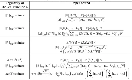
Table 1: Estimates proved by means of Malliavin-Stein techniques

Regularity of Upper bound

the test functionh

kh_{kLi p}is finite _|E[h(G)]₋E[h(X)]_{| ≤} kh_{kLi p}pE[(1_{− 〈}DG,₋D L−1_G〉

H)2]

khkLi pis finite |E[h(G1, . . . ,Gd)]−E[h(XC)]| ≤

kh_{kLi pk}C−1_kopkC_k1_op/2qPd_i,j=1E[(C(i,j)_{− 〈}DG_i,₋D L−1_G

j〉H)2]

kh_{kLi p}is finite _|E[h(F)]₋E[h(X)]_{| ≤} khkLi p(

p

E[(1_{− 〈}DF,−D L−1F〉L2_(µ))2] +R

Zµ(dz)E[|DzF|

2

|D_zL−1F_|])

h_∈C2(Rd) _|E[h(F₁, . . . ,F_d)]₋E[h(X_C)]_{| ≤} khkLi pis finite khkLi pkC−1kopkCk1op/2

qPd

i,j=1E[(C(i,j)− 〈DFi,−D L−1Fj〉L2_(µ))2]

M₂(h)is finite +M₂(h) p

2π

8 kC −1_k3/2

op kCkop

R

Zµ(dz)E

 

‚ _d P

i=1

|D_zF_i| Œ2‚ _d

P

i=1

|D_zL−1F_i| Œ



4.2

Stein’s method versus smart paths: two tables

In the two tables below, we compare the estimations obtained by the Malliavin-Stein method with those deduced by interpolation techniques, both in a Gaussian and Poisson setting. Note that the test functions considered below have (partial) derivatives that are not necessarily bounded by 1 (as it is indeed the case in the definition of the distances d2 and d3) so that the L∞ norms

of various derivatives appear in the estimates. In both tables, d _≥ 2 is a given positive integer. We write (G,G₁, . . . ,G_d) to indicate a vector of centered Malliavin differentiable functionals of an isonormal Gaussian process over some separable real Hilbert space H (see [12] for defini-tions). We write (F,F₁, ...,F_d) to indicate a vector of centered functionals of Nˆ, each belonging to domD. The symbols D and L−1 stand for the Malliavin derivative and the inverse of the Ornstein-Uhlenbeck generator: plainly, both are to be regarded as defined either on a Gaussian space or on a Poisson space, according to the framework. We also consider the following Gaussian random elements: X _{∼ N}(0, 1), X_{C ∼ Nd}(0,C) and X_{M ∼ Nd}(0,M), where C is a d_×d posi-tive definite covariance matrix andM is ad×dcovariance matrix (not necessarily positive definite).

In Table 1, we present all estimates on distances involving Malliavin differentiable random variables (in both cases of an underlying Gaussian and Poisson space), that have been obtained by means of Malliavin-Stein techniques. These results are taken from:[9](Line 1),[11](Line 2),[17](Line 3) and Theorem 3.3 and its proof (Line 4).

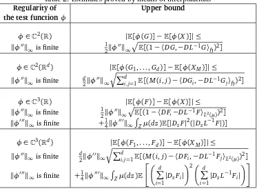
Table 2: Estimates proved by means of interpolations

Regularity of Upper bound

the test functionφ

φ∈C2(R) _|E[φ(G)]₋E[φ(X)]_{| ≤} kφ′′k∞is finite 12kφ′′k∞

p

E[(1_{− 〈}DG,₋D L−1_G〉 H)2]

φ∈C2(Rd) _|E[φ(G₁, . . . ,G_d)]₋E[φ(X_M)]_{| ≤} kφ′′k∞is finite d2kφ

′′_k ∞

qPd

i,j=1E[(M(i,j)− 〈DGi,−D L−1Gj〉H)2]

φ∈C3(R) _|E[φ(F)]₋E[φ(X)]_{| ≤} kφ′′k∞is finite 12kφ

′′_k ∞

p

E[(1_{− 〈}DF,₋D L−1_F〉

L2_(µ))2] kφ′′′k∞is finite +14kφ′′′k∞

R

Zµ(dz)E[|DzF|

2₍

|D_zL−1F_|)]

φ∈C3(Rd) _|E[φ(F1, . . . ,Fd)]−E[φ(XM)]| ≤

kφ′′k∞is finite d2kφ′′k∞ qPd

i,j=1E[(M(i,j)− 〈DFi,−D L−1Fj〉L2_(µ))2] kφ′′′k∞is finite +14kφ′′′k∞

R

Zµ(dz)E

 

‚

d

P

i=1|

D_zF_i|

Œ2‚ _d P

i=1|

D_zL−1F_i|

Œ 

from Theorem 4.2 and its proof.

Observe that:

• in contrast to the Malliavin-Stein method, the covariance matrix M is not required to be positive definite when using the interpolation technique,

• in general, the interpolation technique requires more regularity on test functions than the Malliavin-Stein method.

5

CLTs for Poisson multiple integrals

In this section, we study the Gaussian approximation of vectors of Poisson multiple stochastic inte-grals by an application of Theorem 3.3 and Theorem 4.2. To this end, we shall explicitly evaluate the quantities appearing in formulae (10)–(11) and (15)–(16).

Remark 5.1(Regularity conventions). From now on, every kernel f ∈L2_s(µp)is supposed to verify both Assumptions A and B of Definition 2.8. As before, given f ∈ L2_s(µp_{), and for a fixed z ∈ Z,}

we write f(z,_·) to indicate the function defined on Zp−1 as(z₁, . . . ,z_p−1)_7→ f(z,z₁, . . . ,z_p−1). The following convention will be also in order: given a vector of kernels(f1, ...,fd)such thatfi∈Ls2(µ

pi_), i=1, ...,d, we will implicitly set

for everyz_∈Zbelonging to the exceptional set (ofµmeasure 0) such that

f_i(z,·)⋆l_r f_j(z,·)_∈/L2(µpi+pj−r−l−2₎

for at least one pair(i,j)and somer =0, ...,pi∧pj−1 andl=0, ...,r. See Point 3 of Remark 2.10.

5.1

The operators

G

_kp,q

and

Ô

G

_kp,q

Fix integersp,q_≥0 and_|q₋p_{| ≤}k_≤p+q, consider two kernels f _∈L2_s(µp)andg_∈L_s2(µq), and recall the multiplication formula (6). We will now introduce an operatorG_kp,q, transforming the func-tion f, ofpvariables, and the functiong, ofqvariables, into a “hybrid” functionG_kp,q(f,g), ofk vari-ables. More precisely, forp,q,kas above, we define the function(z₁, . . . ,z_k)_7→G_kp,q(f,g)(z₁, . . . ,z_k), fromZk intoR, as follows:

G_kp,q(f,g)(z₁, . . . ,z_k) =

p∧q

X

r=0

r

X

l=0

1_{(p+q−r−l=k)}r!

‚

p r

Œ ‚

q r

Œ ‚

r l

Œ â_{f ⋆}l

rg, (18)

where the tilde∼ means symmetrization, and the star contractions are defined in formula (4) and the subsequent discussion. Observe the following three special cases: (i) when p = q = k = 0, then f and g are both real constants, and G0,0₀ (f,g) = f _×g, (ii) when p = q _≥ 1 and k = 0, then G₀p,p(f,g) = p!〈f,g〉L2_(µp₎, (iii) when p = k = 0 and q > 0 (then, f is a constant), G0,₀p(f,g)(z₁, ...,z_q) = f _×g(z₁, ...,z_q). By using this notation, (6) becomes

I_p(f)I_q(g) =

p+q

X

k=|q−p|

I_k(G_kp,q(f,g)). (19)

The advantage of representation (19) (as opposed to (6)) is that the RHS of (19) is anorthogonal sum, a feature that will greatly simplify our forthcoming computations.

For two functions f _∈ L_s2(µp) and g _∈ L2_s(µq), we define the function (z₁, . . . ,z_k) _7→

Ô

G_kp,q(f,g)(z1, . . . ,zk), fromZkintoR, as follows:

Ô

G_kp,q(f,g)(_·) =

Z

Z

µ(dz)G_kp−1,q−1(f(z,_·),g(z,_·)),

or, more precisely,

Ô

G_kp,q(f,g)(z₁, . . . ,z_k)

=

Z

Z

µ(dz)

p∧_Xq−1

r=0

r

X

l=0

1(p+q−r−l−2=k)r!

× ‚

p−1

r

Œ ‚

q−1

r

Œ ‚

r l

Œ

å

f(z,_·)⋆l

rg(z,·)(z1, . . . ,zk)

=

p∧q

X

t=1

t

X

s=1

1(p+q−t−s=k)(t−1)! ‚

p₋1

t−1

Œ‚

q₋1

t−1

Œ‚

t₋1

s−1

Œ áf ⋆s

Note that the implicit use of a Fubini theorem in the equality (20) is justified by Assumption B – see again Point 3 of Remark 2.10.

The following technical lemma will be applied in the next subsection.

Lemma 5.2. Consider three positive integers p,q,k such that p,q_≥1and_|q₋p_{| ∨}1_≤k_≤p+q₋2

(note that this excludes the case p =q =1). For any two kernels f ∈L2_s(µp) and g ∈ L_s2(µq), both verifying Assumptions A and B, we have

Z

Proof. We rewrite the sum in (20) as

Ô

Note that the Cauchy-Schwarz inequality

n

5.2

Some technical estimates

As anticipated, in order to prove the multivariate CLTs of the forthcoming Section 5.3, we need to establish explicit bounds on the quantities appearing in (10)–(11) and (15)–(16), in the special case of chaotic random variables.

Definition 5.3. The kernels f _∈ L2_s(µp), g_∈ L_s2(µq) are said to satisfyAssumption Cif either p=

q=1, ormax(p,q)>1and, for every k=_|q−p| ∨1, . . . ,p+q−2,

Z

Z

 

ÈZ

Zk

(G_kp−1,q−1(f(z,_·),g(z,_·)))2_dµk



µ(dz)<∞. (23)

Remark 5.4. By using (18), one sees that (23) is implied by the following stronger condition: for everyk=_|q−p| ∨1, . . . ,p+q−2, and every(r,l)satisfyingp+q−2−r−l=k, one has

Z

Z

 

ÈZ

Zk

(f(z,_·)⋆l

r g(z,·))2dµk



µ(dz)<∞. (24)

One can easily write down sufficient conditions, on f and g, ensuring that (24) is satisfied. For instance, in the examples of Section 6, we will use repeatedly the following fact: if both f and g

verify Assumption A, and if their supports are contained in some rectangle of the typeB_×. . ._×B, withµ(B)<∞, then (24) is automatically satisfied.

Proposition 5.5. Denote by L−1 the pseudo-inverse of the Ornstein-Uhlenbeck generator (see the Ap-pendix in Section 7), and, for p,q_≥1, let F=I_p(f)and G=I_q(g)be such that the kernels f _∈L_s2(µp)

and g∈L2_s(µq_{)verify Assumptions A, B and C. If p6=q, then}

E[(a_{− 〈}DF,₋D L−1G_〉L2_(µ))2]

≤ a2+p2

p+_Xq−2

k=|q−p|

k!

Z

Zk

dµk(GÔ_kp,q(f,g))2

≤ a2+C p2

p+_Xq−2

k=|q−p|

k!

p∧q

X

t=1

1_{1≤s(t,k)≤tk}få⋆s_t(t,k)gk2_L2_(µk₎

≤ a2+1 2C p

2

p+_Xq−2

k=|q−p|

k!

p∧q

X

t=1

11≤s(t,k)≤t(kf ⋆ p−t

p−s(t,k)fkL2_(µt+s(t,k)₎× kg⋆q−t

If p=q_≥2, then

E[(a_{− 〈}DF,₋D L−1G_〉L2_(µ))2]

≤ (p!_〈f,g_〉L2_(µp₎−a)2+p2

2_Xp−2

k=1

k!

Z

Zk

dµk(GÔ_kp,q(f,g))2

≤ (p!_〈f,g_〉L2_(µp₎−a)2+C p2

2_Xp−2

k=1

k!

p∧q

X

t=1

1_{1≤s(t,k)≤tk}få⋆s_t(t,k)g_k2

L2_(µk₎

≤ (p!_〈f,g〉L2_(µp₎−a)2

+1 2C p

2 2_Xp−2

k=1

k!

p∧q

X

t=1

1_{1≤s(t,k)≤t}(_kf ⋆p_p−_−st_(t,k) fkL2_(µt+s(t,k)₎× kg⋆q−t

q−s(t,k)gkL2_(µt+s(t,k)₎)

where s(t,k) =p+q₋k₋t for t=1, . . . ,p_∧q, and the constant C is given by

C =

p∧q

X

t=1 –

(t−1)!

‚

p−1

t₋1

Œ ‚

q−1

t₋1

Œ ‚

t−1

s(t,k)₋1

Ϊ2

.

If p=q=1, then

(a− 〈DF,−D L−1G〉L2_(µ))2= (a− 〈f,g〉_L2_(µ))2.

Proof. The casep=q=1 is trivial, so that we can assume that eitherporqis strictly greater than 1. We select two versions of the derivatives D_zF =pI_p−1(f(z,_·))and D_zG =qI_q−1(g(z,_·)), in such a way that the conventions pointed out in Remark 5.1 are satisfied. By using the definition of L−1

and (19), we have

〈DF,−D L−1G〉L2_(µ) = 〈DI_p(f),q−1DI_q(g)〉_L2_(µ)

= p

Z

Z

µ(dz)I_p−1(f(z,_·))I_q−1(g(z,_·))

= p

Z

Z

µ(dz)

p+_Xq−2

k=|q−p|

I_k(G_kp−1,q−1(f(z,_·),g(z,_·)))

Notice that fori6= j, the two random variables

Z

Z

µ(dz)I_i(G_ip−1,q−1(f(z,·),g(z,·)) and

Z

Z

µ(dz)I_j(G_jp−1,q−1(f(z,·),g(z,·)))

are orthogonal inL2(P). It follows that

E[(a_{− 〈}DF,₋D L−1G_〉L2_(µ))2] (25)

=a2+p2

p+_Xq−2

k=|q−p|

E

 

‚Z

Z

µ(dz)I_k(G_kp−1,q−1(f(z,_·),g(z,_·)))

forp₆=q, and, forp=q,

We shall now assess the expectations appearing on the RHS of (25) and (26). To do this, fix an integerkand use the Cauchy-Schwartz inequality together with (23) to deduce that

Z

Relation (27) justifies the use of a Fubini theorem, and we can consequently infer that

E

The remaining estimates in the statement follow (in order) from Lemma 5.2 and Lemma 2.9, as well as from the fact thatkefkL2_(µn₎≤ kfk_L2_(µn₎, for alln≥2.

The next statement will be used in the subsequent section.

that the kernels f_j verify Assumptions A and B. Then, writing q_∗:=min_{q₁, ...,q_d},

Proof of Proposition 5.6. One has that

Z

To conclude, use the inequality

Z