Vol. 17, No. 4, 2002, 420 - 427
EMPIRICAL STUDY OF VOLATILITY PROCESS
ON ERROR CORRECTION MODEL ESTIMATION
Syamsul Hidayat Pasaribu Yayasan AliFA
ABSTRACT
Ada dua tujuan yang ingin dicapai dalam penelitian ini. Pertama, adalah untuk menyelidiki apakah dalam estimasi model koreksi kesalahan atau error correction model (ECM) terdapat proses volatilitas. Jika ternyata ada, maka model estimasi koreksi kesalahan seharusnya diestimasi dengan menggunakan model volatilitas. Hasil empirik estimasi ECM ternyata mengindikasikan adanya proses volatilitas yang ditunjukkan oleh signifikannya pengujian Autoregressive Conditional Heteroscedasticity (ARCH).
Tujuan kedua adalah untuk menentukan model yang paling baik antara estimasi ECM dan estimasi ECM yang diikuti dengan proses volatilitas. Setelah dilakukan estimasi terhadap kedua model tersebut ternyata dapat disimpulkan bahwa estimasi model ECM dengan proses Generalized ARCH (EC-GARCH) lebih baik dibandingkan dengan estimasi model ECM. Sebagai contoh kasus digunkan model estimasi indeks harga saham gabungan di bursa efek Jakarta (BEJ).
Keywords: error correction model, volatility process, GARCH, EC-GARCH.
INTRODUCTION
One the expression in Jakarta stock composite index (JSCI) trend and it volatility is that the possibility of the significant effect of LQ45 index movements. Recent studies on volatility models, especially in the stock market volatility models used univariate expression (Bollerslev and Kroner, 1992; Bollerlev, et al, 1994). Univariate model does not explain the economic variable relations as economic theory expression. Thus, we should create model that explains the relations among the economic variables. One of the most popular dynamic models is error correction model (ECM). This model widely used in dynamic modeling because its properties explained the short-run effects as well as long-run effects.
The main purpose of the paper is to search for the volatility process on ECM. If there are volatility processes in ECM empirical
estimation, we should estimate it with volatility process model. For this purpose, most of empirical studies used Generalized Autoregressive Conditional Heteroscedasticity (GARCH) specification (Engle, 1982; Bollerslev, Engle, Nelson, 1994; Engle, 2000; Engle and Patton, 2001). Thus, we may estimate the ECM by applying GARCH model. Finally, we compare the empirical estimation of ECM model and ECM with GARCH model and choose the superior model by several criteria model selection such as Akaike Information Criterion (AIC) and Schwarz Information Criterion (SIC).
II of this study describes the data and the time series properties (such as, unit root test, co-integration test and error correction model) employed to assess the LQ45 Index and JSX Composite Index (JSX-CI) relationship and its empirical results. Section III provides GARCH processes on error correction model and the
We built the economic relationship bet-ween LQ45 index and JSX-CI in econometric model. Let LQ45 index as independent variables and JSX-CI as dependent variable. LQ45 index consists of 45 shares, which are high in liquidity, and is selected through a set of criteria (see www.jsx.co.id for detail information). LQ45 Index was first introduced on February 24th, 1997. July 13th, 1994 is used as the basis for the index calculation, valued at 100. The premiere selection used market data from the date of July 1993 to June 1994 and resulted in 45 issuers which covered 72% of the total market capitalization and 72,5% of the regular market’s total transaction value. That is why the index has major role of stock trading and composite index movements in JSX and treats as independent variables in this research. The single model of long-run relationship ln(LQ45), respectively. The original data source of the variables is the JSX, however obtained from the database of the Accounting Research Center of Faculty of Economics
Gadjah Mada University. The sample size is taken to be 1451 and all calculations in this research use Eview Version 3.
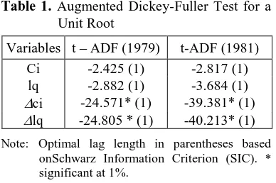
Unit Root Test
We start the analysis by establishing the time series properties of individual variables. The aim here is simply to show that the variables are integrated of the same order. The sampling distribution of OLS estimator is not well behaved if the disturbance is non-stationary. If a unit root present, it is essential to first difference the variables, thereby eliminating the unit root and achieving stationarity before attempting to estimate the model. augmented Dickey-Fuller tests are performed with trend and intercept in level data, but
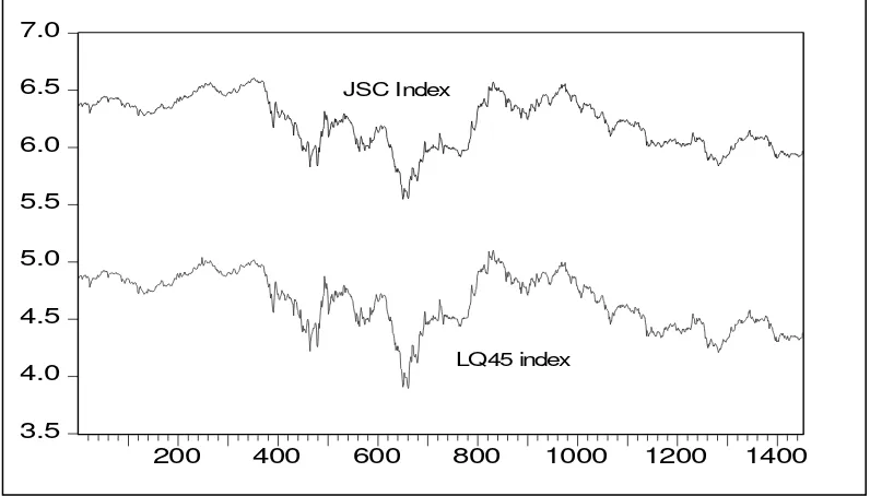
Co-integration and Error Correction Model One way to identify the co-integrating relationship between ci and lq is by identified the time series paths a long of observations. This identification is shown in Figure 1. It is
not mistake to say that ci's path movements similar to lq's path movements. This figure tells us that maybe there is long run relationship (co-integration) between those variables.
Figure 1. Trend of Composite Index and LQ45 Index on JSX, February, 1st, 1996-December, 28th, 2001 (in natural logarithm)
Given a group of non-stationary series or random walks stochastic processes (note both the variables I(1)), we may be interested in determining whether the series are co-integrated, and if they are, an identifying the long-run equilibrium relationship. Engle and Granger (1987) pointed out that a linear combination of two or more non-stationary series might be stationary. If such a stationary, or I(0), linear combination exists, the non-stationary, time series are said to be co-integrated. The stationary linear combination is called the co-integrating equation and may be interpreted as a long-run equilibrium relation-ship between the variables.
If there is a linear combination of the variables such as equation (1), or we can write that equation as,
ut = cit - -lqt (2) where, is constant term, and find that ut is I(0) or stationary, then we say that the variables ci and lq are co-integrated. We can say it as before, they are on the same wavelength. In the language of co-integrating theory, a regression such as equation (1) is known as a co-integrating regression and the parameter and are known as the co-integrating parameters.
3.5 4.0 4.5 5.0 5.5 6.0 6.5 7.0
200 400 600 800 1000 1200 1400
JSC Index
There are number methods for testing for co-integration that have been proposed (see Engle and Granger (1987), Gonzalo (1994)). Two simple methods are (1) the ADF test on ut estimated from co-integrating regression and (2) the co-integrating regression Durbin Watson (CRDW) test (Sargan and Bhargava, 1983). The co-integrating regression results is,
cit = 1.956641 + 0.914550 lqt (3) (0.056824)* (0.12139)*
R2-adjusted = 0.956; CRDW = 0.013; ADF (1976) = -1.936; ADF (1981) = -1.621 and values in parentheses are robust standard error of Newey-West (1987) Heteroskedasticity and Auto-correlation Consistent (HAC) Covariance with truncation lags=7. The asterisks indicate the coefficients estimated significant at 1% critical level. The results of equation (3) show that CRDW statistics and ADF (1981) indicate no co-integrating regression while the ADF (1976) indicates there is co-integrating equation at least 5% critical level. This results show us that the residual of equation (3) is stationary or I(0).
Having established that composite index is co-integrated with LQ45 index, we moved onto examining the associated error correction mechanism that describes the short-run dynamics. The general model of error correction model could be specified as following equation (see Thomas, 1997).
cit =1 ECt-1 +
EC represents the residuals from co-integrating equation (3). The coefficients j imply the impacts of LQ45 index to Composite Index in the short run. We will use general specification approach to set the best estimation of equation(4). The estimation of ECM yielded the 8.135, SIC = -8.120. LM is a serial correlation test, RESET is a functional form test, and ARCH is ARCH test, AIC is Akaike Information Criterion, and SIC is Schwarz Information Criterion. Numbers in parentheses denote standard errors of Newey-West consistent HAC with truncation lags=7, while those in brackets denote p-values. The two asterisks indicate that the coefficient is significant at 5% critical level.
Heteroskedasti-city) models. ARCH models are specifically designed to model and forecast conditional variances. The variance of the dependent variable is modeled as a function of past values of the dependent and independent (exogenous) variables (Engle, 2001).
ARCH models were introduced by Engle (1982) and generalized as GARCH (Generalized ARCH) by Bollerslev (1986). These models are widely used in various branches of econometrics, especially in financial time series analysis. Bollerslev, Chou, and Kroner (1992) and Bollerslev, Engle, and Nelson (1994) provided the recent surveys of theory and empirical of ARCH models.
A popular member of volatility models is the GARCH(p,q) model. Following the results of equation (5), the GARCH(p,q) model of the equation (4) becomes, explosive and to guarantee positive variances. If i and/or j have negative values, they will not have economic meaning. However, with the inclusion of one period lag value of volume in the equation this condition may fail, despite it will be tested empirically. Those models can be estimated via maximum likelihood once a distributions of the innovations, t, has been specified.
A commonly employed assumption is that the innovations are normal distribution (Gaussian). Bollerslev and Wooldridge (1992) had proven that maximum likelihood estimated
the GARCH model assuming Gausian errors were consistent even if the true distribution of innovations is not Gaussian. The usual standard errors of estimators were both consistent when the assumption of Gaussianity of the errors was violated. Bollerslev and Wooldridge had provided a method for obtaining consistent estimated of those.
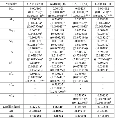
Table 2 provides the empirical estimation of some GARCH(p,q) classes. First, we used GARCH specification for GARCH(3,0), GARCH(2,0), GARCH(2,1) and GARCH(1,1). We may chose the suitable model based on tree selection criteria, namely, Loglikelihood Ratio (LR), Akaike Information Criterion, and Schwarz Information Criterion. Based on those criteria, we choosed the GARCH(3,0) specification as the suitable model.
Evaluating the empirical model of GARCH(3,0), we use residual tests based on Correlogram–Q-statistics of the standardized residuals. We use lags to include equal to 20, and show that Q-statistics equal to 14.155 [p-value=0.823] and it is not significant. Thus, we can make a conclusion that the mean equation is correctly specified.
We do the test of residual based on correlogram squared residuals for remaining ARCH in the variance equation and to check the specification of the variance equation. If the variance equation is correctly specified, all Q-statistics should not be significant. The test statistics for include 20 lags, is 1.0614 [p-value =1.000]. Again, it is not significant.
Table 2. Re-estimated Equation (5) allows GARCH Process
Variables GARCH(2,0) GARCH(3,0) GARCH(2,1) GARCH(1,1)
ECt-1 -0.005460 -0.004328 -0.004534 -0.004082
(0.001635)* (0.001808)** (0.001801)** (0.001911)** ((0.002581))** ((0.002498))*** ((0.002592))*** ((0.002277))***
lqt 0.794228 0.794396 0.797712 0.799931
(0.002425)* (0.002070)* (0.002542)* (0.002610)* ((0.007976))* ((0.009043))* ((0.008493))* ((0.009550))*
lqt-1 0.065273 0.0041169 0.027536 0.001621
(0.016279)* (0.020741) (0.022098) (0.023413) ((0.101578)) ((0.036258)) ((0.072184)) ((0.083212))
cit-1 -0.041177 0.031844 -0.003872 0.026313
(0.022524)*** (0.024762) (0.027689) (0.028722) ((0.109059)) ((0.047153)) ((0.087006)) ((0.103899))
7.91E-06 7.02E-06 4.54E-06 2.89E-06
(1.05E-07)* (1.21E-07)* (3.77E-07)* (2.84E-07)* ((3.01E-06))* ((2.86E-06))** ((2.18E-06))** ((1.26E-06))**
2
t-1 0.181054 0.194491 0.178255 0.309271
(0.029201)* (0.028264)* (0.027180)* 0.031848 ((0.139491)) ((0.140099)) ((0.154387)) ((0.202144))
2
t-2 0.591893 0.100134 0.338985 -
(0.032708)* (0.032441)* (0.035939)* - ((0.351613))*** ((0.099216)) ((0.319336)) -
2
t-3 - 0.515035 - -
- (0.037882)* - -
- ((0.251700))** - -
2
t-1 - - 0.351979 0.594282
- - (0.044844)* ((0.033913))*
- - ((0.112003))* ((0.069884))*
Log likelihood 6122.333 6153.40 6136.766 6117.695
AIC -8.440763 -8.48226 -8.459305 -8.434361
SIC -8.415262 -8.45312 -8.430161 -8.408860
In the conditional mean equation, the error correction variable (ECt-1) and lqt have significant impacts to composite index at least 5% and 1% critical level while lqt-1, and cit-1 have no significant values. The coefficient of EC is now corrected to be –0.004 rather that – 0.009 in ECM model. The other coefficients also have been corrected to become 0.794, 0.004, and 0.032 for variables lqt, lqt-1, and
cit-1, respectively instead the values of those coefficients in ECM model.
Figure 2 and 3 show us the actual values, fitted values, and residual values of empirical estimation of ECM and EC-GARCH(3,0) model. We may use Akaike Information Criterion and Schwarz Information Criterion
for model selection. Based on these criteria, all support to choose the EC-GARCH(3,0) over ECM. Thus, the second purpose of this research had been confirmed.
Figure 2. The Actual, Fitted, and Residual Values of Error Correction Model
Figure 3. The Actual, Fitted, and Residual Values of EC-GARCH(3,0) Model -0.06
-0.04 -0.02 0.00 0.02 0.04
-0.2 -0.1 0.0 0.1 0.2
200 400 600 800 1000 1200 1400
Residual Actual Fitted
-0.06 -0.04 -0.02 0.00 0.02 0.04 0.06
-0.2 -0.1 0.0 0.1 0.2
200 400 600 800 1000 1200 1400
CONCLUSION
The purposes of this paper have been proven above. The error correction model not always produce constant variance (homoscedasticity) and the results of this research have proven that such as model produces non-constant variance (heteroscedasticity). These results imply that model is following volatility processes. Thus, we had estimated the ECM with GARCH processes (EC-GARCH model), and produced the better estimation than its ECM by several criteria model selection. Finally, both purposes of this research had been confirmed.
REFERENCE
Dickey, D.A. and W.A. Fuller., (1979), Distribution of the Estimators for Autoregressive Time Series with a Unit Root, Journal of the American Statistical Association, 74, 427–431.
____, (1981), Likelihood Ratio Statistics for Autoregressive Time Series with a Unit Root, Econometrica, 49, 1057-1072. Engle, Robert F., (1982), Autoregressive
Conditional Heteroskedasticity with Estimates of the Variance of U.K. Inflation, Econometrica, 50, 987–1008. Engle, Robert F., (2001), GARCH 101: The
Use of ARCH/GARCH Models in Applied Econometrics, Journal of Economic Perspectives, 4, 157-168.
Engle, Robert F. dan Andrew J.P., (2001), What Good is a Volatility Model?, Quantitative Finance, 1, 237-245.
Engle, Robert F. and C.W.J. Granger., (1987), Co-integration and Error Correction: Representation, Estimation, and Testing, Econometrica 55, 251–276.
Bollerslev, T., (1986), Generalised autore-gressive conditional heteroscedasticity, Journal of Econometrics, 31, 307-27. Bollerslev, Tim and Jeffrey M. Wooldridge.,
(1992), Quasi-Maximum Likelihood Estimation and Inference in Dynamic Models with Time Varying Covariances, Econometric Reviews, 11, 143–172. Bollerslev Tim, Ray Y. Chou, and Kenneth F.
Kroner., (1992), ARCH Modeling in Finance: A Review of the Theory and Empirical Evidence, Journal of Econo-metrics, 52, 5–59.
Bollerslev, Tim, Robert F. Engle and Daniel B. Nelson., (1994), ARCH Models, in Chapter 49 of Handbook of Econometrics, Volume 4, North-Holland.
Gonzalo, J., (1994), Five Alternative Methods of Estimating Long-Run Equilibrium Relationships, Journal of Econometrics, 60, 203-233.
Sargan, J.D and A.S. Bhargava., (1983), Testing Residual from Least Squares Regression for Beeing Generated by the Gaussian Random Walk, Econometrica, 51, 153-174.
Thomas, R.L., (1997), Modern Econometrics: An Introduction, Addison-Wesley.