INCREMENTAL PRINCIPAL COMPONENT ANALYSIS BASED OUTLIER
DETECTION METHODS FOR SPATIOTEMPORAL DATA STREAMS
Alka Bhushan*, Monir H. Sharker, Hassan A. Karimi
Geoinformatics Laboratory, School of Information Sciences, University of Pittsburgh, PA15260, USA - [email protected], (mhs37, hkarimi)@pitt.edu
KEY WORDS: Outlier Detection, Incremental Principal Component Analysis, Spatiotemporal Data Streams
ABSTRACT:
In this paper, we address outliers in spatiotemporal data streams obtained from sensors placed across geographically distributed locations. Outliers may appear in such sensor data due to various reasons such as instrumental error and environmental change. Real-time detection of these outliers is essential to prevent propagation of errors in subsequent analyses and results. Incremental Principal Component Analysis (IPCA) is one possible approach for detecting outliers in such type of spatiotemporal data streams. IPCA has been widely used in many real-time applications such as credit card fraud detection, pattern recognition, and image analysis. However, the suitability of applying IPCA for outlier detection in spatiotemporal data streams is unknown and needs to be investigated. To fill this research gap, this paper contributes by presenting two new IPCA-based outlier detection methods and performing a comparative analysis with the existing IPCA-based outlier detection methods to assess their suitability for spatiotemporal sensor data streams.
*
Corresponding author, Current affiliation: GISE Lab, Department of Computer Science and Engineering, Indian Institute of Technology Bombay, Mumbai, India-400076
1. INTRODUCTION
Spatiotemporal data streams obtained from sensors placed across geographically distributed locations have been used in various applications such as environmental monitoring, object tracking and traffic monitoring (Gama and Gaber, 2007). A key challenge in such applications is that sensors may produce data streams at a very fast rate leading to numerous computational challenges (Aggarwal, 2013a). Typically, data collected from these sensors is sent to a central server through a communication network. Thus, such data is prone to outliers that can result from instrumental error, sudden environmental changes, and communication error. An Outlier in a dataset is
defined as “a data point which is significantly different from
other data points" (Barnett and Lewis, 1994). For any meaningful analysis of data, it is essential to detect these outliers in real-time.
Various methods for outlier detection in spatiotemporal data have been presented in the literature (Hill and Minsker, 2010;
O’Reilly et al., 2014; Zhang et al., 2010). Most of these methods either do not work on streaming data or incur large computational cost. Recently, forecasting based outlier detection method has been proposed for spatiotemporal streaming data (Appice et al., 2014). However, this method is not scalable due to large computational cost. A detailed survey on generic outlier detection techniques is beyond the scope of this paper. Interested readers can see (Aggarwal, 2013b; Chandola et al., 2009; Sadik and Gruenwald, 2013) for literature survey. In this work, we focus on Principal Component Analysis (PCA) based outlier detection methods.
PCA is one of the most popular techniques for detecting outliers in various applications such as industrial processes (Li et al., 2000), environmental sensors (Harkatet al., 2006; Harrou et
al.,2013), distributed sensor networks (Chatzigiannakis and Papavassiliou, 2007), and high dimensional data (Ding and Kolaczyk, 2013). Most PCA-based models for outlier detection operate in batch mode (Chatzigiannakis and Papavassiliou, 2007; Harrou et al., 2013; Harkat et al., 2006), where the model is first trained using training data and is then used to test the remaining data for outliers. As such, these models are time invariant. However, for streaming data, the following data characteristics may change with time (Li et al., 2000): (i) mean and covariance, and (ii) correlation structure which results in increase or decrease in number of principal components. The
data which changes with time is also called “non-stationary
data”. For the model to adapt to the change, it needs to be
computed either at frequent intervals or when change occurs. Finding the correct time interval to avoid unnecessary computation or detecting the change is a challenging task. Another requirement is that the entire data needs to be stored for updating the model and model should be updated in real time.
To address these challenges, several Incremental PCA (IPCA) methods have been proposed (Li et al., 2000; Papadimitriou et al., 2005; Zhao and Yuen, 2006). These variants update the models incrementally and require minimal storage. However, most of these IPCA models have been used either for finding outliers in non-spatiotemporal data or for finding correlation among the spatiotemporal data streams. Hence, there is a need to evaluate the suitability of IPCA-based outlier detection methods for spatiotemporal data streams. In this article, we propose two new IPCA-based outlier detection methods by extending the existing batch PCA-based outlier detection methods and compare them with the existing IPCA-based outlier detection methods (Li et al., 2000) to assess their suitability for spatiotemporal sensor data streams. As part of the evaluation, we apply these methods to two environmental
datasets each consisting of a set of geographically distributed sensors. We introduce various point outliers in these datasets and compare the performances of the methods in terms of rate of correct outlier detection as well as false alarm (wrongly identified outliers) rates. The time complexity of these methods is also analysed. Based on these comparisons, an appropriate IPCA method is recommended for detecting outliers in spatiotemporal datasets.
The rest of the paper is structured as follows. Section 2 describes PCA and IPCA methods. Section 3 discusses outlier detection methods based on PCA. Problem definition, the proposed methods and comparative framework are described in Section 4. Section 5 discusses the comparison experiments and the results. Conclusions are presented in Section 6.
2. PCA AND INCREMENTAL PCA METHODS
2.1 PCA
PCA is a statistical multivariate analysis technique which captures the correlation among variables and represents the data into a new set of few variables capturing the maximum variance. These variables are denoted as principal components (PCs) and each PC is a linear combination of original variables (Jolliffe, 2002). The vector of coefficients of this linear combination defines the corresponding principal direction. PCA can be formulated as an optimization problem which minimizes the reconstruction error as:
min
�n×k,∥�∥=∑ ∥ ��− − � ��− ∥
�
�=
(1)
where ��ℜ� is a vector of measurements at time �, � is number of time points for which data is currently available, ℜ�×� is a matrix with its columns being the principal directions, � is the number of PCs, and is the mean vector of the data.
The data characteristics such as mean and correlation structure change with time due to the change in the environment. In such cases, principal directions and hence PCs need to be updated to adapt to the change in real time. Two popular updating methods are:
Batch mode: PCs are updated at either fixed time interval or when change is detected. This method requires: (a) storage of past data and (b) identification of a correct interval size at which such updates are performed.
Incremental mode: PCs are updated at each time instance. Unlike the batch methods, these methods do not require storage of the past data or determination of the interval size. As a result, this method is fast and preferred for streaming data. This method is denoted as Incremental PCA (IPCA) method.
In this article, we focus on Incremental PCA as described below.
2.2 Incremental PCA Methods
Various incremental methods for computing PCs, when all the data is not simultaneously available, have been proposed (Li et al., 2000; Li, 2004; Zhao and Yuen, 2006; Weng et al., 2003;
Papadimitriou et al., 2005). These can be categorized as covariance based and covariance free methods, and are summarized next.
2.2.1 Covariance Based Method: In this method, PCs are updated at each time instance using updated covariance matrix. There are two approaches in using covariance matrix. In the first approach, data covariance matrix is used where initial covariance matrix is computed using training data (Li et al., 2000) and then it is updated at each time instance using current data sample. Then the updated covariance matrix is used in computing new PCs. A number of methods for detecting the number of PCs (�) have been proposed (Li et al., 2000). The most popular method is cumulative percent variance (CPV) which measures the percent of variance captured by the � PCs corresponding to � largest eigen values. Efficient methods, such as Lanczos method (Golub and Van Loan, 1996), can be used for computing high PCs. High PCs and their respective eigen values are sufficient for detecting outliers (Li et al., 2000). The time complexity of Lanczos-based method is � � , where � is the number of sensors, � is the dimension of lanczos matrix and � ≪ �. In this approach, previous PCs are not used in computing new PCs.
In the second approach (Halla et al., 2002; Li, 2004), previous PCs and current data sample are used in computing a reduced covariance matrix, which in turn is used in computing new PCs. The advantage of this approach is that the size of covariance matrix is much smaller than the dimension of the data since only a few PCs are used. However, the main drawback with this approach is that the number of PCs always remains same and thus it cannot deal with the change in correlation structure of the data.
We use the first approach for our comparison and denote it as COV.
2.2.2 Covariance Free Method: A covariance free method has been proposed for computing PCs incrementally (Papadimitriou et al., 2005; Weng et al., 2003). This method updates the number of PCs as well as the principal directions guaranteeing that reconstruction error is predictably small.
We use the approach given in (Papadimitriou et al., 2005) for our comparison and denote it as COVF. The time complexity of this method is �� , where � is the number of PCs selected for PCA.
3. OUTLIER DETECTION
PCA-based methods to find outliers can be broadly categorised into statistics-based methods and oversampling methods.
3.1 Statistics-Based Methods
Statistics-based methods have been widely applied in detecting outliers in environmental data (Harkat et al., 2006; Harrou et al., 2013) and process monitoring (Li et al., 2000). The most popular statistics are:
(a) Q-statistic: It is also known as squared prediction error or squared reconstruction error (SRE). It measures the amount of variance not captured by the current PC model for the current (at time �) sample �� and is computed as:
�= ��� − �− �−� �� (2)
where �− ∈ ℜ�×�is a matrix of principal directions corresponding to � high PCs at time � − . The sample’s Q -statistic is computed using the previous PCs and is compared to a threshold value (Li et al., 2000). This threshold is obtained analytically based on the distribution of the Q-statistic. If the error is above this threshold, then the current sample is considered as an outlier and is reported for further investigation.
A threshold on SRE can also be computed using mean of previous SRE values (Chatzigiannakis and Papavassiliou, 2007). We label this method as SRE method.
(b) � Statistic: It is used to measure the variance captured in the current model and is defined as:
�� = ��� �− Λ�−− �−� �� (3)
where Λ�− = ���� , , … , � is the diagonal matrix of the � largest eigen values at time � − . Computation of this statistic also needs updated eigen values. � statistic has a chi-squared distribution with � degrees of freedom. The threshold value of � statistic is �� � for a given level of significance �. A sample is considered to be an outlier if the value of � statistic is more than the threshold value.
For our comparison to be presented later on, we use Q-statistic for the COV method (denoted as COV-Q) as given in (Li et al., 2000) and the SRE method for COVF method (denoted as COVF-SRE). To our knowledge, SRE method has been used with batch PCA only (Chatzigiannakis and Papavassiliou, 2007); not in incremental mode.
3.2 Oversampling
In the oversampling method (Lee et al., 2013), the current sample is replicated many times and oversampled PCA is applied on all replicated data. The idea is to amplify the effect of an outlier by replicating the sample many times and then measure the variation in the first PC. This would make it easier to find outlier even for a large data set, but this method has not been proposed for IPCA.
For our comparison, we modify the method to make it suitable for IPCA and use this method along with COVF for outlier detection. This method is denoted as COVF-Oversamp.
4. PROBLEM DEFINITION AND METHOD
In this article, we consider point outliers which are spikes in the sensor values at discrete points of time. The problem is defined as follows: given a collection of temporal streams obtained from a set of n sensors, placed across various geographical locations, the objective is to monitor the series and detect point outliers in real-time, i.e., upon arrival of data.
We consider our dataset outliers free and insert various point outliers in the dataset. This will help us to know the places of point outliers. To compare the COV-Q, COVF-SRE and COVF-Oversamp methods, we use the following steps for each method:
1. Compute data mean, PCs, number of PCs (�), and threshold value for outlier detection using the first � + data samples. For COV-Q, compute eigen values as well.
2. For each sample ��= [�� �� … ���]� that arrives at time � > � +
a. Subtract mean value from ��
b. Compute SRE for COV-Q and COVF-SRE, and variation between oversampled PC and first PC for COV-Oversamp.
c. If the value is above a threshold, report for outlier and assign the original value to �� d. Update the mean value, PCs, � and
threshold value.
For time varying data, it is important to ignore the old data to capture the most recent behaviour. In step d above, while updating the mean, an exponential forgetting factor with < <�−� < can be used (Li et al., 2000; Papadimitriou et al., 2005). It can also be considered as a tuning parameter which depends on how fast the system changes.
For our experiments, we tried different values of and set = .9 which resulted in the smallest average reconstruction error for each method.
Figure 2. Measurements and mean of chlorine data (Blue: sensor 1, red: sensor 2 and green: sensor 3) Figure 1: Measurements and mean of AQI data
Figure 2: Measurements and mean of chlorine data (blue: sensor 1, red: sensor 2, green: sensor 3)
5. EXPERIMENTS
Since COV method given in (Liet al., 2000) and COVF method in (Papadimitriou et al., 2005) have not been compared before, first we compare them based on number of PCs required in each method, reconstructed values, and reconstruction error obtained from each method. Then, outlier detection methods are compared.
5.1 Datasets
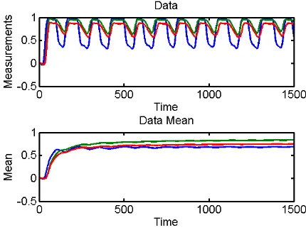
We used the air quality index (AQI) dataset which is publicly available from central Environmental Protection Agency (EPA) repository in USA (EPA, 2011). EPA has placed sensors to measure pollutants across locations all over USA. The data is collected on hourly basis. Each sensor measures air pollutants at regular intervals and sends the measurement to the central data repository. AQI measures the quality of air which is computed based on the quantity of pollutants measured at each location at each given instance. From amongst 3000 sensors, 81 sensors from one geographically chosen area are selected for the experiments. The data and its mean are shown in Figure 1. In this figure, time is on the x-axis and values corresponding to all sensors are on the y-axis.
We also used the chlorine dataset presented in (Papadimitriou et al., 2005) which contains chlorine concentration level across 166 junctions tracking the flow of water at each pipe in a network. The dataset contains 4310 timestamps collected over 15 days at 5 minutes interval. The data is periodic and has slight phase shift due to the time taken for fresh water to flow down the pipes from reservoirs. The data and its mean from first 3 sensors are shown in Figure 2.
5.2 Results on AQI Data
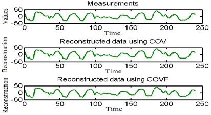
5.2.1 Comparison of Both the Methods: Both COV and COVF methods require one PC each for representing the data. The average of squared reconstruction error using both the methods is same, i.e., 0.488. In Figure 3, the original values centred at mean are shown in the first plot and reconstructed values using COV and COVF methods are shown in next plots. From the figure, it can be seen that the reconstructed values match the original measurements quite well.
Figure 3: Reconstructed values and original measurements: AQI data
5.2.2 Comparison of Outlier Detection Methods: It is assumed that the data does not have any outliers. To set thresholds and compute initial PCs for different methods, the dataset was divided into training and test sets. The first 82 values from time point 1 to 82 are considered as training data
set and the rest of 158 values are considered as testing dataset. In the testing data set, outliers were randomly introduced at 10% of the points in randomly chosen sensors. Further, the magnitudes of the outliers were randomly chosen to be between 0.1-0.2 of the corresponding sensor values. This resulted in a total of 16 outliers. Outlier detection results from the three methods are shown in Table 1. From the results, it can be seen that all outliers have been detected by COV-Q and COV-SRE. However, COV-SRE detects smaller number of false alarm instances than COV-Q.
5.3 Results on Chlorine Data
5.3.1 Comparison between Methods: As seen in Figure 2, chlorine data has slight phase shift in the measurements of each sensor. For this, a slightly different implementation of COVF method is used for training the initial model than the one used for the AQI data. Here, since COVF updates the vectors at each time instance and mean of the data is periodic using forgetting factor 0.9, we update the training model in every iteration by using the updated mean in every training instance. Initially, the COV method requires the number of PCs to be between 3-5 and this number then fluctuates between 2-3 while the COVF method requires 6 PCs throughout the process. The average of SRE using both methods is same, which is 0.004203. The original values centred at mean are shown in the first plot and the reconstructed values obtained from COV and COVF are shown in next plots in Figure 4. From the figure, it can be seen that the reconstructed values match the original measurements quite well.
Methods Correct detection instances
False alarm instances
Cov-Q 244 313
CovF-SRE 330 349
CovF-Oversamp 7 78
Table 2: Outlier detection results: Chlorine data
Figure 4: Reconstructed values and original measurements: chlorine data (blue: sensor 1, red: sensor 2)
Comparison of Outlier Detection Methods: Similar to the previous dataset, it is assumed that the data does not have any
Methods Correct Detection Instances
False Alarm Instances
COV-Q 16 43
COVF-SRE 16 24
COVF-Oversamp
15 26
Table 1: Outlier detection results: AQI data
outlier. To set thresholds and compute initial PCs for different methods, the first 167 data values are considered as training set and the rest of 4143 values are considered as testing dataset. In the testing dataset, 10% of points in randomly chosen sensors are considered as outliers and values equal to its mean value at that time instance plus 3 times of standard deviation are considered. This resulted in a total 433 outliers. Outlier detection results obtained from the three methods are shown in Table 2. From the results, it can be seen that the number of correct number of instances is less than the number of outliers present in the data. Also, the number of false alarms is more than the number of correct number of instances. These results show that the presented techniques may not work well on such type of data where data from each sensor has a phase shift.
6. CONCLUSIONS
Based on the experiment results, it can be seen that the COV-SRE method outperforms the other methods for spatiotemporal data in terms of correct detection instances and running time complexity. Use of this method is proposed and this can be taken as an initial recommendation for detecting outliers in spatiotemporal data streams. Further, detailed comparison for datasets with a much larger number of sensors is required. For such situations, sensors can be clustered based on their spatial locations and point outliers can then be identified locally in each cluster. The presented techniques assume that the data comes to central server at regular time interval and does not consider the missing data. Extensions to scenarios where this assumption does not hold can also be considered as future work.
REFERENCES
Aggarwal, C.C., 2013a. Managing and mining sensor data . Springer.
Aggarwal, C.C., 2013b. Outlier Analysis. Springer.
Appice A., Guccione P., Malerba D. and Ciampi A., 2014. Dealing with temporal and spatial correlations to classify outliers in geophysical data streams. Information Sciences, 285, pp. 162-180.
Barnett, V. and Lewis, T., 1994. Outliers in statistical data (Vol. 3). New York: Wiley.
Chandola, V., Banerjee, A. and Kumar, V., 2009. Anomaly detection: A survey. ACM Computing Surveys, 41(3), pp.15:1- 15:58.
Chatzigiannakis, V. and Papavassiliou, S., 2007. Diagnosing anomalies and identifying faulty nodes in sensor networks. IEEE Sensors J., 7(5), pp. 637-645.
Ding, Q. and Kolaczyk, E., 2013. A compressed PCA subspace method for anomaly detection in high-dimensional data. IEEE Trans. Inf. Theory, 59(11), pp. 7419-7433.
Environmental Protection Agency, 2011. EPA-AQS, Retrieved June 6, 2012, http://www.epa.gov/ttn/airs/airsaqs/
Gama, J. and Gaber, M., 2007. Learning from Data Streams Processing Techniques in Sensor Networks. Springer.
Golub, G. and Van Loan, C., 1996. Matrix Computations (3rd
Edition ed.). The Johns Hopkins University Press.
Gupta, M., Gao, J. and Han, J., 2014. Outlier detection for temporal data: A survey. IEEE Trans. Knowl. Data Eng., 26(9), pp. 2250-2267.
Halla, P., Marshallb, D., and Martinb, R., 2002. Adding and subtracting eigenspaces with eigenvalue decomposition and singular value decomposition. Image and Vision Computing, 20, pp. 1009–1016.
Harkat, M., Mourot, G. and Ragot, J., 2006. An improved PCA scheme for sensor FDI: Application to an air quality
monitoring network. Journal of Process Control, 16, pp. 625- 634.
Harrou, F., Nounou, M. and Nounou, H., 2013. Detecting Abnormal Ozone Levels using PCA-based GLR Hypothesis Testing. IEEE Symp. on Computational Intelligence and Data Mining.
Hill J.D. and Minsker S.B., 2010. Anomaly detection in streaming environmental sensor data: A data-driven modelling approach. Environmental Modelling & Software, 25, pp. 1014-1022.
Jolliffe, I., 2002. Principal Component Analysis. New York: Springer.
Lee, Y., Yeh, Y. and Wang, Y., 2013. Anomaly detection via online oversampling principal component analysis. IEEE Trans. Knowl. Data Eng., 25(7), pp. 1460–1470.
Li, W., Yue, H. H., Valle-Cervantes, S. and Qin, S. J., 2000. Recursive PCA for adaptive process monitoring. Journal of Process Control, 10, pp. 471-486.
Li, Y., 2004. On incremental and robust subspace learning. Pattern Recognition, 37, pp. 1509 – 1518.
O’Reilly C., Gluhak A., Imran A.M. and Rajasegarar S. 2014.
Anomaly detection in wireless sensor networks in a non-stationary environment. IEEE Comm. Surveys & Tutorials, 16(3), pp. 1413-1432.
Papadimitriou, S., Sun, J., and Faloutsos, C. 2005. Streaming Pattern Discovery in Multiple Time-Series. Proc. of the 31st VLDB Conference, pp. 697-708.
Sadik, S., and Gruenwald, L., 2013. Research issues in outlier detection for data streams. ACM SIGKDD Explorations Newsletter, 15(1), pp. 33-40.
Weng, J., Zhang, Y. and Hwang, W., 2003). Candid covariance- free incremental principal component analysis. IEEE Trans. Pattern Anal. Mach. Intell., 25(8), pp. 1034-1-40.
Zhao, H. and Yuen, P., 2006. A Novel Incremental Principal Component Analysis and Its Application for Face Recognition. IEEE Transactions on Systems, Man and Cyberbetics Part B: Cybernetics, 36(4).
Zhang Y., Meratnia N. and Havinga P. 2010. Outlier detection techniques for wireless sensor networks: A survey. IEEE Comm. Survey & Tutorials, 12(2), pp. 159-170.