HOMOLOGICAL PERSISTENCE FOR SHAPE BASED CHANGE DETECTION
BETWEEN DIGITAL ELEVATION MODELS
Bruno Vallet
IGN, Laboratoire MATIS 73 avenue de Paris 94165 Saint-Mand´e, FRANCE
[email protected] recherche.ign.fr/labos/matis/∼vallet
Commission III/3
KEY WORDS:Change detection, Digital Elevation Model, shape, persistence, multilevel
ABSTRACT:
Digital Elevation Models provide an accurate description of scenes allowing change detection by radiometric independence measure-ments. The height information gives access to the changes in the 3D shape of a scene occurring between two dates. In this paper, a procedure to extract meaningful changes is proposed based on analysing this shape variation. Instead of filtering a difference map, a multilevel analysis of the difference map based on the theory of persistence is developed to make such analysis independent from a choice of threshold values.
1 INTRODUCTION
1.1 Context
Change detection from aerial or spatial images is a major stake for accelerating and automatizing of geographical databases. Such databases are becoming larger, more complete and more accurate, so the task of keeping them up to date is becoming ever more challenging. In this study, we consider change detection based solely on Digital Elevation Models (DEMs). We have made this choice because we are interested in finding only where the ge-ometry of the scene has changed, not only its radige-ometry. This is much simpler as radiometric differences may come from many other sources than a change in the scene geometry: change in lighting conditions, in object color, in acquisition conditions (dif-ferent viewpoint), etc. The drawback of this choice is that we will be very dependant on the quality of the DEM used to detect the changes. In particular, we will not be able to sort easily between actual changes and DEM errors.
1.2 Related works
Change detection has often been performed in order to update an existing geographic database, for instance of buildings, in which case the data at the former date is this database, and aerial/satellite imagery at the later date. This is out of the scope of this paper, which focusses on purely DEM to DEM comparison (without re-quiring such a database), so we refer to the detailed performance analysis of (Champion et al., 2011) on such approaches.
Most existing change detection between DEMs rely on the fol-lowing simple steps:
1. Resample the two DEMs in a common geometry (if they are not already). The height information comes either from Aerial Laser Scanning (ALS) or photogrammetric dense match-ing usmatch-ing aerial images.
2. Compute the difference map between the DEMs in this com-mon geometry. (Kuo-hsin et al., 2006) proposes to simply give this map to an operator for visual interpretation.
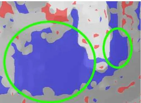
Figure 1: Constructions (blue) and destructions (red) obtained by thresholding a DEM difference map. Two separate constructions (circled in green) are merged by the choice of a low threshold. The resulting component has a low compactness while the indi-vidual real changes were highly compact, which may result in their rejection based on shape analysis.
3. Threshold the difference map
4. Filter the resulting binary mask based on the shapes of its components
detec-tion. Finally the uncertainty on the height given by the individual DEMs can be estimated to refine the study of their difference in the context of topographic survey of sediment budgets (Wheaton et al., 2010). The spatial variability of elevation is then estimated through a fuzzy inference system then this estimate is modified based on the spatial coherence of height variation.
Such approaches suffer from a major drawback: The results highly depend on the choice of the threshold used to binarize the differ-ence map. High thresholds tend to miss some significant changes, leading to high under detection rates. Conversely, low thresholds tend to merge different changes into a single change with very complex shape (Figure 1) that risks rejection by a compactness criteria while the individual changes were compact enough. The resulting detection will also be highly undersegmented.
Classification may be used in two different ways for change de-tection:
1. Classifying the data at the two dates and comparing the clas-sifications, as proposed by (Chaabouni-Chouayakh et al., 2010)
2. Posing the change detection problem as a classification prob-lem
Two very innovative recent works take the second choice:
1. (Gu´erin et al., 2012) poses the problem of change detec-tion as a labelling problem with a data attachment term and a regularization term, which solution is found by dynamic programming. Thus unlike (Chaabouni-Chouayakh et al., 2010), compactness is not used to filter out components but is a prior to enforce that the components found are compact.
2. (Tian et al., 2013) proposes to merge segmentations of the DEM at the two dates and classify the resulting segments using various indicators.
Finally, we can cite a very different approach: in the case of aerial laser scanning, (Hebel et al., 2011) proposed to work directly in 3D (instead of a 2.5D DEM) by voxelizing space and using the intersection of laser rays with such voxels to decide wether thay are occupied. Changes are then located by finding conflicts be-tween such occupancy computed for two different acquisitions using Dempster-Shafer evidence theory.
1.3 Method overview
The approach that we propose studies the morphology of changes in order to make the detection independent from the choice of an arbitrary (and hard to tune) threshold, thus to avoid the afore-mentioned issues. Homological persistence will be used to study changes at all the levels when significant changes happen in or-der to automatically choose the threshold the most appropriate to their analysis.
As with classical approaches, we start by filtering a difference map between the DEMs at the two dates and splitting this dif-ference map (Section 2.1). Splitting separates positive and neg-ative components of the difference maps (potential constructions and destructions), resulting in very large components, which only serves to cut the area of interest into smaller areas that will be analysed independently. This is preferable over cutting the area in rectangular blocks because this way we ensure that no change will overlap two blocks (changes will be strictly contained in
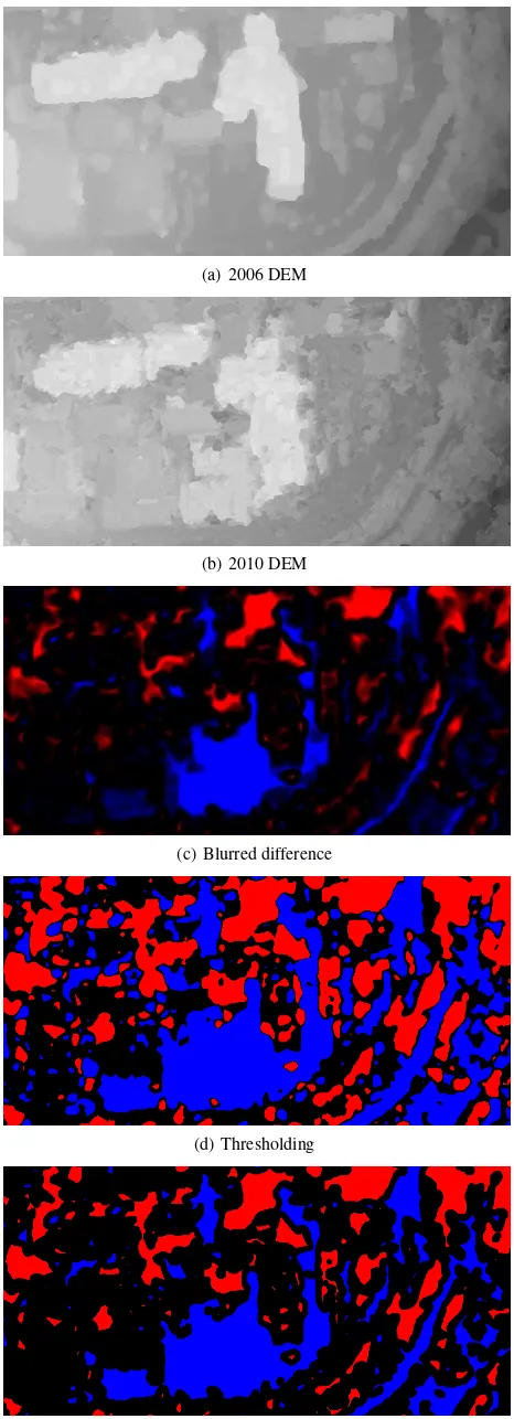
(a) 2006 DEM
(b) 2010 DEM
(c) Blurred difference
(d) Thresholding
(e) Erosion
these components). Each component is then analysed using the theory of homological persistence in order to study the compact-ness of all possible topological subcomponents. The theory of homological persistence is briefly presented in Section 2.2, the definition of a compactness criterion is given in Section 2.3 and the application of both to shape based change detection in Sec-tion 2.4. Finally results are given and discussed in SecSec-tion 3 and conclusions drawn in Section 4.
2 METHOD
2.1 Filtering
We propose to filter the difference map both before and after split-ting as shown in Figure 2. A general idea that we push forward in this paper is that the full shape of the change needs to be anal-ysed. By ”shape of the change” we mean both the altimetric shape (shape of the difference map over the area of the detected change) and planimetric (shape of the detected change area as seen on a map). Blurring the DEM difference before splitting allows to give more importance to small changes with high alti-metric difference. This is performed by convolution of the DEM difference with a Gaussian (Figure 2(c)) which standard devia-tion should be adapted to the DEM resoludevia-tion (typically 4 times the pixel size). After this blurring, the DEM difference is split (Figure 2(d)) into positive and negative components. Construc-tions (∆>0) and destructions (∆<0) can be separated in this step. Finally, a morphological erosion is performed (Figure 2(e)) to remove thin differences often occurring near building edges. The resulting components should not be interpreted as changes but as areas of potential changes that will be analysed in further steps using homological persistence (Section 2.2) and generalized compactness (Section 2.3).
2.2 Homological Persistence
Homological persistence is a very general study of the evolution of the topology of the level sets of functions as the level varies. We will only present here the special case of 2D functions over the real space (f :R2 →R) and only study the first homology group (of order 0), which represent the connectedness of compo-nents. In 2D there is also a second group (of order 1) representing the loops. For the general theory of homological persistence, we point the interested reader to (Cohen-Steiner et al., 2005).
Homological persistence relies on detecting topological events that occur when there is no strict 1-to-1 mapping (by inclusion) between the connected components of:
fa={x∈R2|f(x)≤a∈R} (1)
between two different levelsa1 < a2. In our special case, this may only happen when:
1. A component appears betweena1anda2(minimum off).
2. Two components merge betweena1anda2(saddle point of
f).
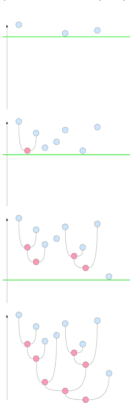
For a functionf defined over a set S of pixelsp, this will be done by constructing apersistencetree. Each node and leaf of the tree is a connected componentsCi⊂Idefined by the set of its pixels and having a unique identifieri. The tree is built by pro-gressively adding all pixelspin descending or ascending order of
f(p)and maintaining an identifier mapId(p). Updating the tree
when adding a pixelpdepends on the number of different exist-ing active components in its neighbourhood (number of different identifiers in the neighbourhood ofpin the identifier mapi):
1. 0: creation of a new active componentCicontaining only
pand settingId(p) =i. Such components are leafs of the persistence tree, they do not have ancestors.
2. 1: growing the neighbouring componentCiby addingpto its set of pixels and settingId(p) =i.
3. n >1: merging the neighbouring componentsCi1, ..., Cin
by creating a new componentCjcontaining all the pixels of all the merged components. SetId(p) = jandId(q) =
j∀q∈Ci1∪...∪Cin. DeclareCi1, ..., Cinas ancestors of Cj. They are now inactive (they won’t change any more) as their identifiers have all been replaced byjin the identifier map.
This construction finishes when all the pixels in S have been added. At that point, there is only one active component con-taining all the pixels ofS. The process is illustrated in Figure 3 where the nodes are placed at the creation level of the corre-sponding component.
The persistence tree represents the topological structure of the level sets of the function, and its construction is parameter-free. When we analyse the DEM difference, the changes that we want intuitively a change detection method to find can be at any level of this tree. Thus we will analyse all the nodes of the tree in order to find the changes of interest, based on several geometric criteria, for instance:
1. Area of the change: number of pixels of the component
2. Maximum, median or average height of the change: maxi-mum, median or average∆zbetween pixels of the compo-nents, or equivalently level difference between the analysed node and the highest leaf over it.
3. Compactness: see Section 2.3.
The first three indicators are very easy to compute (they can be updated each time a pixel is added to a component) and are vari-ous indicators of the size (both altimetric and planimetric) of the change. In order to make our geometric analysis finer, we pro-pose, as (Chaabouni-Chouayakh et al., 2010), to use a compact-ness operator. Compared to this work, our contribution is double:
1. The compactness operator is used to analyse nodes at all the levels of the persistence tree instead of a single arbitrary level.
2. We define a generalized compactness to overcome some lim-itations of the classical compactness.
2.3 Generalized Compactness
(Chaabouni-Chouayakh et al., 2010) use the classical compact-ness indicator defined by:
C(C) = 2
p
πA(C)
P(C) ∈[0,1] (2)
whereAandPare the area and perimeter of the componentC. It is maximum (1) for disks, close to 0 for very complex/elongated
shapes, and 0 for 1D shapes (that have a perimeter but null area). These properties are useful to filter out elongated and complex components, but suffers a strong limitation in our case where components are rasterized (represented by a set of pixels). Indeed rasterization implies that smaller components are more compact than larger ones (it is hard to be complex or elongated is you have few pixels). In other terms, because the pixel size is fixed, com-pactness is sensitive to scale. To overcome this limitation, we propose the following ”generalized” compactness :
Cα(C) =
s
2(2π)αA(C)
P(C)α+1 (3)
the constants being chosen such that a disk of radius r has a compactness ofr(1−α)/2. Theα= 1case is the classical com-pactness criterion which favours small components. Conversely,
α= 0favours too much large components soαshould be chosen in the[0,1]interval.
2.4 Application to shape based change detection
We now need an indicator of what is a good geometry for a change, and consider that the answer to this question is very ap-plication dependent. In our case, we were mainly interested in building, so we chose a quality estimator of the form:
Q(C) =C0.5(C)∆avz (C)
C0.5has similar values for small compact components and larger more complex components, which characterizes well the planime-try of buildings, and the second term favours changes for which the altimetric difference is high. This quality criteria combines the quality of the planimetric and altimetric shape of the potential changes.
The selection of components in the persistence tree based on quality criterionQis then done in a greedy manner:
1. ComputeQfor each node of the tree
2. While the quality of the best componentQ(Cbest)is above a threshold:
(a) AddCbestto the list of detected changes
(b) RemoveCbest, all its ancestors (components contain-ing Cbest) and successors (components included in
Cbest) from the tree
(c) Find the new best component in the rest of the tree.
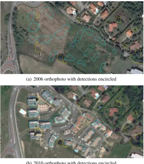
This algorithm allows for a much finer geometric analysis of changes than without using the multilevel approach based on per-sistence. For instance, the two components of our running exam-ple are well separated as shown on Figure 4(a) without requiring a threshold tuning.
(a) On our running example: the two components circled in Figure 1 are well separated
(b) On the vegetation: most complex components are filtered out. Only the components with compact shapes remain and will need a vegetation mask to be filtered out.
Figure 4: Result of the greedy search: all potential changes are encircled in red (destructions) and blue (constructions), selected changes are in yellow (destructions) and cyan (constructions).
3 RESULTS AND DISCUSSION
A performance study of this algorithm has been conducted on two test areas covering around2km2near the cities of Phoenix (USA) and Toulouse (France). The ”Phoenix” area covers an industrial zone so most of its area is covered with industrial buildings and parking lots with vehicles of various sizes. The ”Toulouse” area is in the suburbs and contains a wide variety of typologies: individ-ual and collective housing, large buildings (hospital and school), forest, fields,... The data available on Phoenix was panchromatic satellite imagery: Ikonos in 2008 with 80cm GSD and World-view2 in 2011 with 46cm GSD. For Toulouse, we used 25cm GSD aerial photographs from 2006 and 70cm GSD Pl´eiades satel-lite images from 2010. The four DEMs have been made us-ing the MicMac software (Pierrot-Deseilligny and Paparoditis, 2006), with a standard parameterization.
Results are satisfactory even in difficult cases. Figure 5 shows the correct detection of new buildings, and Figure 6 shows that even (large) vehicles groups can be detected. All the
signifi-(a) 2006 orthophoto with detections encircled
(b) 2010 orthophoto with detections encircled
Figure 5: Constructions correctly detected over the Toulouse area by our method (cyan=constructions, yellow=destructions).
(a) 2008 panchromatic image with detections highlighted
(b) 2011 panchromatic image with detections encircled
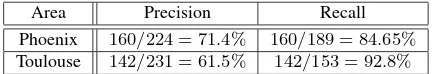
Area Precision Recall Phoenix 160/224 = 71.4% 160/189 = 84.65%
Toulouse 142/231 = 61.5% 142/153 = 92.8%
Table 1: Performance of our algorithm on the two selected areas around Toulouse
cant changes are detected, and the compactness criteria elimi-nates most artefacts. False alarms mainly come from errors in the input DEMs. An interpreter (specialized in change detection from satellite imagery) has validated the results of our algorithm (separating true and false detections) and noted the areas where real changes had not been detected, which allowed us to compute thePrecision(ratio of good detections over the total number of detections) andRecall(ratio of good detections over total number of real changes) which are given on Table 1 for the two areas.
Thanks to the NDVI based vegetation mask, most false alarms in vegetation have been removed. Many false alarms remain in ar-eas where vegetation is not detected consistently between the two dates. It is often hard to know if this is really due to a change be-tween vegetation and non vegetation classes that is not interpreted as meaningful by the operator or to errors in the vegetation masks. Most of the other false alarms come from errors in the DEM com-putation, and in particular around discontinuities that are often smoothed by the regularization term of the surface reconstruction method. This problem is even increased in our case where the satellites were viewing the scene under a rather high angle (away from NADIR). Things are even worse when the viewing direction is very different at the two dates (which was the case on Phoenix), or when the acquisition typology is different (aerial vs spatial in Toulouse). These considerations are general to all DEM based change detection approaches and not only ours. Finally, it has to be noted that the results were evaluated by professional image interpreters, for which the notion of meaningful changes, in an operational definition, is often quite far from varying heights as we try to define change in this work. Thus many false alarms and missed detections come from this differences of point of view. A tree replaced by bare ground will be detected by our algorithm but often omitted by the interpreter.
Concerning the parametrization of the method, the only parame-ters to tune are the two parameparame-ters of the filtering, theα parame-ter of generalized compactness and the threshold on quality. The first two are very standard while the last two are very specific to our method and define what the correct shape for a change is. The main contribution of this paper is not the shape analysis that uses these two parameters (even if the generalized compactness is novel and useful) but the (parameter free) persistence tree con-struction.
4 CONCLUSIONS AND FUTURE WORK
Homologic persistence and the notion of persistence tree allow for a multi-level analysis of the geometry of changes that is not sensitive to the choice of a threshold. Generalized compactness has proved a useful geometric indicator if the change detection fo-cuses mainly on buildings as it allows for the rejection of complex shapes without favouring smaller components too much. The re-sults are highly satisfactory and lead us to think that this algo-rithm could be used for production purposes, as long as the qual-ity of the DEMs used is sufficient. Enhancing DEM qualqual-ity is therefore the best lead for improvement. Obviously, the method will also perform better is the DEMs have been acquired in sim-ilar conditions (time of day and year, viewing angle, resolution, same sensor, ...) and if the same method (and same parameters for this method) is used.
Future work on the method itself will probably focus on a more global optimization (rather than greedy search) to select the op-timal subset of components from the persistence tree, and to in-tegrate other cues than purely geometric ones (using edges ex-tracted from the images and image based classifications at the two dates). Finally, we could exploit the results to use our persistence tree concept along with a supervised learning method instead of simply thresholding a quality criterion.
REFERENCES
Chaabouni-Chouayakh, H., Krauss, T., dAngelo, P. and Reinartz, P., 2010. 3d change detection inside urban areas using different digital surface models. In: Paparoditis N., Pierrot-Deseilligny M., Mallet C., Tournaire O. (Eds), IAPRS, Vol. XXXVIII, Part 3B.
Champion, N., Boldo, D., Pierrot-Deseilligny, M. and Stamon, G., 2011. 2d change detection from satellite imagery: Perfor-mance analysis and impact of the spatial resolution of input im-ages. In: Proc. of the IEEE International Geoscience and Remote Sensing Symposium (IGARSS), Vancouver, Canada.
Cohen-Steiner, D., Edelsbrunner, H. and Harer, J., 2005. Stabil-ity of persistence diagrams. In: Proceedings of the twenty-first annual symposium on Computational geometry, SCG ’05, ACM, Pisa, Italy, pp. 263–271.
Gu´erin, C., Binet, R. and Pierrot-Deseilligny, M., 2012. D´etection des changements d’´el´evation d’une sc`ene par imagerie satellite st´er´eoscopique. In: Reconnaissance des Formes et Intel-ligence Artificielle, RFIA 2012, Lyon, France.
Hebel, M., Arens, M. and Stilla, U., 2011. Change detection in ur-ban areas by direct comparison of multi-view and multi-temporal als data. In: Proceedings of the 2011 ISPRS conference on Pho-togrammetric image analysis, PIA’11, Springer-Verlag, Munich, Germany, pp. 185–196.
Iovan, C., Boldo, D. and Cord, M., 2008. Detection, characteriza-tion and modeling vegetacharacteriza-tion in urban areas from high resolucharacteriza-tion aerial imagery. EEE Journal of Selected Topics in Applied Earth Observations and Remote Sensing 1(3), pp. 206–213.
Kuo-hsin, H., Liu, J., Cheng, D. and Yu, M., 2006. Terrain change detection combined photogrammetric dem. Perspective c, pp. 1– 6.
Pierrot-Deseilligny, M. and Paparoditis, N., 2006. A multireso-lution and optimization-based image matching approach: An ap-plication to surface reconstruction from spot5-hrs stereo imagery. In: International Archives of Photogrammetry, Remote Sensing and Spatial Information Sciences, Vol. 36 (Part 1/W41), Ankara, Turkey.
Sasagawa, A., Watanabe, K. N. S., Koido, K., Ohno, H. and Fu-jimura, H., 2008. Automatic change detection based on pixel-change and dsm-pixel-change. In: The International Archives of the Photogrammetry, Remote Sensing and Spatial Information Sci-ences, Vol. XXXVII. Part B7, Beijin, China, pp. 1645–1650.
Tian, J., Reinartz, P., dAngelo, P. and Ehlers, M., 2013. Region-based automatic building and forest change detection on cartosat-1 stereo imagery. {ISPRS}Journal of Photogrammetry and Re-mote Sensing 79(0), pp. 226 – 239.