*Fax: 0171-222-1435. The author would like to thank Martin Weale, Jayasri Dutta, David Miles and Kjetil Storesletten for their help as well as all the participents of CORE symposium on General Equilibrium Models. The research was funded from E.S.R.C. grant No. R000236788.
E-mail address:[email protected] (J.A. Sefton)
A solution method for consumption decisions
in a dynamic stochastic general
equilibrium model
J.A. Sefton*
National Institute of Economic and Social Research, 2, Dean Trench Street, Smith Square, London SW1P 3HE, UK
Abstract
In this paper we describe a numerical solution of the consumer's life-cycle problem based on value function iteration. The advantage of our approach is that it retains the versatility of the value function iteration approach and achieves a high degree of accuracy without resorting to the very computationally burdensome task of calculating a very"ne grid. There are two innovations, the"rst is not to discretise the state space but e!ectively to allow the states to take any value on the real line by using two di!erent third-order interpolation algorithms: bicubic spline for extrapolation and interpolation on the edge of the grid and the faster cubic convolution interpolation for inside the grid. The second is to compute a pair of nested grids, one coarse and one "ne. The "ne grid is used to calculate the consumption paths of the majority of individuals, and the coarse grid to catch only the few with very high incomes. We shall discuss our approach in relation to those already in the literature. We shall argue that value function iteration approach is probably the most#exible and robust way to solve these problems. We shall show that our implementation achieves a high degree of accuracy, using a modi"ed den Haan and Marcet simulation accuracy test, without comprising signi"cantly on speed. ( 2000 Elsevier Science B.V. All rights reserved.
JEL classixcation: C68; D58
Keywords: Computational methods; Value function iteration; Hetereogeneous agent models
1. Introduction
In this paper we describe a numerical solution of the consumer's life-cycle problem based on value function iteration. The advantage of our approach is that it retains the versatility of the value function grid approach: it can easily accommodate increasing complexities such as liquidity constraints, margins between interest rates on lending and borrowing, means-tested bene"ts, uncer-tain life length etc. At the same time it achieves a high degree of accuracy without resorting to the computationally burdensome (and therefore time-consuming task) of calculating a very"ne grid. The motivation for solving this consumer problem e$ciently and accurately is to be able to solve a general equilibrium model with as near as possible a continuum of consumers.
We have made two innovations to the basic value function iteration approach as described in Taylor and Uhlig (1990, p. 2). The"rst is e!ectively to allow the states of the problem to lie anywhere on the real line rather than at a set of discrete grid points by using two di!erent third-order interpolation algo-rithms: bicubic spline for extrapolation and interpolation on the edge of the grid and the faster cubic convolution interpolation for inside the grid. The second is to compute a pair of nested grids; a coarse one and a"ne one. The
"ne grid is used to calculate the consumption paths of the majority of indi-viduals, and the coarse grid to catch the few very wealthy, or productive or just plain lucky ones.
Any numerical solution algorithm must be assessed according to its accuracy, speed,#exibility and robustness. We discuss in detail these concepts and show how the performance of other algorithms in the literature can be assessed according to these criteria. We argue that our algorithm compromises slightly on speed, but gains in both#exibility and robustness. We assess its accuracy in detail by using the den Haan and Marcet test of simulation accuracy. This is a powerful test which has been used previously by Den Haan and Marcet (1994) and Campbell and Koo (1997) to rank solutions to stochastic steady-state problems according to their accuracy. We have adapted this test slightly so that now its results also include an absolute measure of accuracy as well as a com-parative one. These tests all suggest that our solution algorithm attains a very high degree of accuracy.
robustness and"nally Section 5 tests the accuracy of our algorithm using the den Haan and Marcet (1990) test.
2. The general equilibrium model
The economy consists of nindividuals (in the simulation results presented here there are 5000 individuals). Each individual is uncertain about his life-span. The life of a individual will start at age 20, q"0, and will always be less than or equal to 90 years, q"70. We shall denote the conditional prob-abilities of dying at the end of periodqgiven that the individual has survived to the beginning of that period as pqimplying of course that p70"1. There-fore the probability that an individual will survive anotheriyears from period
q,/
q,i, is simply the cumulative product of the conditional probabilities
/
q,i"<qj`i/q~1(1!pj). We shall use the standard notation, cq, yq and wq
to denote the individual's consumption, gross wages during the period and wealth at the beginning of any period, respectively. Individuals make their consumption decisions so to maximise their utility over the rest of their expected lifetime. Utility can be derived either directly from their tion or from a bequest made at death. The utility resulting from any consump-tion stream is described by a constant elasticity of substituconsump-tion (CES) utility function
;
q"
A
EqA70~+qi/0
/
q,i((1!d)c(1~q`ic)#dpq`i(Bwq`i`1)(1~c))di
BB
1@(1~c), (1)
where the parameters d, 1/c andB are the discount factor, the intertemporal elasticity of substitution and the bequest motive, respectively. Thus we have modelled the bequest motive of the parent as being independent of the expected consumption of its child. Probably the most common utility function in the literature is;1~c
q ; however, we have taken a monotonic transformation of this
particular utility function. This transformation implies in the absence of uncer-tainty that the value function is linear in total wealth, that is human plus non-human capital. This is desirable, as the easiest functions to interpolate and extrapolate are linear ones. As we generalise our model the value function will no longer be linear, but at least, in some sense, we have minimised these deviations from linearity.
An individual's spending is limited by the constraint that on death he must not be in debt. As there is a "nite probability of dying in any period, this constraint actually implies that at all times an individual's wealth must always be positive or zero, so
w
where
wq
`1"(1#rq)wq#yq!cq. (3)
If we denote the maximum achievable level of utility at time qby the value function, by<
q(wq,yq), then the value function must satisfy the following Bellman
equation:
This is the equation we solve backwards iteratively to calculate the optimal consumption path for every individual.
As well as facing uncertainty about their life-span, individuals face consider-able uncertainty about their future labour income,y
t. This is de"ned as equal to wages or salaries times human capitals
tht, where the future aggregate level of wages is known but human capital is expected to follow the following stochastic process,
where both e and e8 are uncorrelated innovation processes drawn from the distributionse&N(kt,p) ande&N(k8t,p8t), respectively, andhMtis the economy's mean level of human capital. This is the model of income dynamics proposed in Dutta et al. (1997) and estimated for the United Kingdom on the data of income dynamics in the British Household Panel Survey. The model is a synthesis of two popular models of income dynamics in the literature; the mover-stayer (Blumen et al., 1955) and random walk models (Champernowne, 1953; Hart, 1976). Whenk
t"pt"0 the model reduces to the mover-stayer model. In this
case, there is a probability of (1!h) that an individuals income stays constant and a probabilityhthat it moves, in which case the new level of income is drawn from a lognormal distribution. The model generalises on this structure by allowing for the possibility that if an individual stays his income follows a random walk rather than remaining constant. In the modelhwas estimated as function of income: the probability of an individual moving diminishes as his income increases. The mean of the innovation processeande8was also allowed to vary with age so as to describe the&hump-shaped' income pro"le one sees over a typical life.
1Meade (1976, pp. 173}175) suggested that this is a cause of the high level of dispersion in the wealth holdings of households.
where capital depreciates at a constant rate,d, every year so that if aggregate consumption is denotedC
t, then
K
t`1"(1!d)Kt#>t!Ct.
The problem is therefore to"nd the prices, the interest rate and the wage rate where
so that the demand and supply sides are in equilibrium. This problem therefore resembles in structure most of the general equilibrium models in the literature that have generalised away from the representative consumer.
The model of the income dynamics has an important consequence, that the value function is not homogeneous in its two arguments because the expected variance in income is related to its absolute level. Dutta et al. (1997) show that this complexity is necessary, if one is to model e!ectively the distribution of incomes in the United Kingdom. However it is not di$cult to think of other market attributes or imperfections that would imply that consumption depends on the absolute level of income and wealth rather than more simply their ratio. Some examples are the consumption#oor in Hubbard et al. (1994), the means tested bene"t described in Hubbard et al. (1995) or a required minimum level of assets before access to a particular asset market is possible.1
3. Numerical solution algorithms
The general equilibrium model described in the previous section is solved by iterating between the supply and demand side of the economy. First, a set of prices is proposed; given these prices one solves the demand side of the economy for the implied desired level of aggregate wealth and consumption. Given these levels for the aggregate variables, one can then solve the supply side for a new set of implied prices. Now the process can be repeated until a"xed point is found. The convergence of the algorithm can be increased dramatically by introducing some damping in the interest rate iterations.
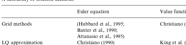
Table 1
A taxonomy of solution methods
Euler equation Value function
Grid methods (Hubbard et al., 1995; Christiano (1990)
Baxter et al., 1990; Attanasio et al., 1995)
LQ approximation Christiano (1990) King et al. (1988)
Parametrized expectations den Haan and Marcet (1990)
2The other principle reason is for analytical simplicity. This motivation cannot be criticised from the computational viewpoint.
3.1. Desirable properties of any solution algorithms
Any numerical solution algorithm is a compromise between the following considerations
(1) Accuracy, (3) Flexibility,
(2) Speed, (4) Robustness.
The"rst point needs little elaboration. Some degree of accuracy is obviously a pre-requisite for the algorithm to be of any use; however it is often di$cult to ascertain precisely the accuracy of the algorithm. We shall discuss this in detail in Section 5.
Speed is always a consideration in this area as general equilibrium models are exceptionally computationally burdensome, and so it is much possible for the solution of a general equilibrium model to take some days to solve. This is one of the reasons that some authors have decided to approximate the non-linear optimisation problem by a Linear Quadratic Gaussian one.2 The "nal two criteria, though slightly more abstract, should also be taken into account in the design phase. A #exible algorithm is one that can solve a wide variety of problems without substantial redesigning. This criterion obviously becomes more important the more experiments the researcher wishes to undertake. Finally, a robust algorithm is an algorithm that has two desirable properties, the
"rst is that it converges from a wide variety of initial guesses, and the second is that an error in one time period does not propagate causing larger errors or even instability later.
3It would of course be possible to solve the Euler equation over di!erent domains of the choice variable where the value function is smooth and then take the maximum over the di!erent domains, but this leads to unacceptable complexity in all but the most simple problems, (Deaton, 1991).
equations. The former is a multivariable minimisation problem whereas the latter involves solving a set of non-linear equation. Press et al. (1993, p. 373) argue that, in terms of their computation burden, the two problems, if well de"ned, are almost identical. However on the basis of both the #exibility and robustness criteria an approach based on solving the Bellman equation must be regarded as superior. To derive the "rst-order conditions, one has to assume di!erentiability of the value function with respect to the choice variable on its closed feasible domain. Therefore one has already assumed away an interesting class of problems where the value function may not be smooth, for example where there is means testing up to some maximum limit, or di!erent rates of interest for borrowing or lending etc.3
The argument concerning robustness is slightly more involved. Solving the consumers'decision problem using the Bellman equation rather than the Euler equation can be shown to be more robust under some very weak conditions. The conditions are the same as those required to guarantee that the value function will tend to some"nite limit as one iterates further back in time. The argument is as follows: if these conditions are satis"ed then we know the value function will tend to the same limit if we iterate backward whatever the initial starting point. Therefore if there is an error in the grid at any point, this error must slowly be attenuated as we iterate back in time. Conversely with the Euler equation approach, we know that under the same conditions that the ratio of consump-tion in any two periods will tend to a constant. Therefore if there is an error in the calculated level of consumption in any period, this will not be attenuated but propagated backwards so that the ratio of the consumption level in any two periods remains roughly constant. The result of the propagation of this error is that when we calculate the consumption path of a consumer by&running'the consumer through our grids, there will be a consistent error in the growth rate of his or her consumption path and not just the levels. This is even though at each point in time the Euler equations are almost satis"ed.
4This drawback though can be removed without too much extra complication by using an exponential linear quadratic approximation as in Whittle (1990).
these models exhibits the property of certainty equivalence and so cannot be used to study precautionary savings.4
We have therefore eliminated all but two of the possible solution techniques. As far as we are aware there as yet been no work be done on parametrising the value function, but there is no reason why this should be any harder than parametrising the expectation of the choice variable as in den Haan and Marcet (1990). Choosing between these two is more di$cult. If the value function were not smooth, then probably the grid method would be preferable because it is clearly di$cult to approximate unsmooth functions with polynomials with any degree of accuracy. However as the number of states increases the grid method becomes computationally very expensive because the number of grid points increases with the power of the number of states. An ideal might be a combination of the two, where the grid dimensions correspond to those states with respect to whom the value function is not smooth. Then at each of these grid points the value function is parametrised with respect to the remaining states with respect to whom it is smooth.
4. Our solution procedure
We have argued that any approach based on Euler-equations is unlikely to be particularly #exible. We now present a grid method approach to solv-ing the value function or Bellman equation. Its principle advantage over a method based on parametrising the value function is that it can cope easily with cases when the value function is not smooth. Its drawback is that as soon as there is more than one state, the computational burden can become insur-mountable. The reason for this is that in the literature, it has always been recommended that to achieve any sort of accuracy it is necessary for the grid to be relatively "nely spaced. The number of points at which the grid is calculated goes up with the power of the number of states. Therefore if one of the domains of the two states are discretised to a 100 points. This can soon mean one is solving 10,000 optimisation problems to calculate a grid for each time period. If each household lives for 100 years, then for a simula-tion of 100 years (where it would be necessary to calculate a new set of grids for those born in each year), we would be solving 1]108 optimisation problems for each solution of the demand side! If one also takes into account that to calculate,E
t<t`1(wt`1,yt`1)(1~c)for each iteration of the optimisation
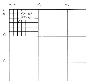
Fig. 1. The layout of the grids.
a algorithm that makes it possible to calculate an accurate solution using a robust and#exible approach.
It is computationally possible to calculate only a coarse grid in a reasonable period of time. We therefore have to make some use of interpolation. Our choice of the structure of the grid is based on the following two general observations which are true for most equilibrium models
1. That the majority of individuals (say about 90%) are clustered in a very small area of the state space.
2. The value function is signi"cantly smoother at the regions of the state space where either the income or wealth of the individual is large or equivalently the value function is large.
We therefore calculate two grids for each time period, a coarse grid for the lower values of the value function and a very coarse grid for the higher values. These two grids were nested so as to provide a continuous coverage of the state space, see Fig. 1. The grid intervals were chosen so that the 90% of individuals would have labour income and wealth holdings falling within the span of the
As both grids were coarse, compared to other algorithms in the literature, we placed considerable reliance on the interpolation routines.
4.1. Interpolation routines
We used two di!erent interpolation routines within our algorithm; a modi"cation of the bicubic interpolation Press et al. (1993) algorithm and the cubic convolution Keys (1981) algorithm. Both are third-order algorithms (by this we mean both will be able to interpolate a third-order polynomial on a regularly space grid with no error), but have very di!erent strengths and weaknesses.
4.1.1. Bicubic spline interpolation
This algorithm has two strengths which we found particularly useful; it can be adapted in order to extrapolate outside the grid, and the grid intervals need not be equal. Its disadvantage is that it is very slow in comparison to cubic convolution. We shall now describe brie#y how we adapted this algorithm so that it could be used e!ectively for extrapolation as well as interpolation. This discussion is done in only one dimension (To interpolate a function in more than a single dimension simply requires that this algorithm be repeated for each dimension). Let the (x
i,yi), i"1.nbe thencouplets of nodes and function values
to be interpolated. The idea behind the algorithm is to"t an!1 cubic splines or polynomials,f
i(x) (fi(x) is the spline on the interval [xi,xi`1]) to each interval
that satis"es the conditions
1. that the spline has the actual grid value at the grid nodes, f
i(xi)"yi and
f
i(xi`1)"yi`1
2. that the"rst di!erential of two splines in adjacent intervals is smooth at the boundary,f@
i(xi`1)"f@i`1(xi`1) andfAi(xi`1)"fAi`1(xi`1).
These conditions in conjunction with a terminal condition for the "rst dif-ferential of the spline on the edge of the grid are su$cient to describe a unique set of splines. However, it is the terminal conditions that must be chosen with care if one is going to able to use these splines to extrapolate outside the grid. Our condition, which is su$cient to determine uniqueness of the splines but
&bends'the splines the least, is to require that the third di!erential of the splines in the penultimate and ultimate intervals are equal, fA@1"fA@
2 andfA@n~2"fA@n~1.
To illustrate why this terminal condition is the most suitable assume for the moment that each spline is described by the polynomial f
i(x)"si#tix#
u
ix2#vix3, and the underlying polynomial is in fact a third-order poly-nomial y"s#tx#ux2#vx3. The interpolating conditions are su$cient to ensure the spline f
by these same conditions the coe$cients s, t, u, of the interpolating spline
f
n~1(x) are also correctly estimated. Our terminal condition, if enforced,
will imply that fA@
n~2"6vn~2"fnA@~1"6vn~1"6v and therefore each spline
will still be a perfect estimate of the underlying polynomial even at the edges of the grid. These splines can therefore be used for extrapolation outside the grid as well as interpolation within the grid.
The polynomial,f
i(x), has the following functional form
f
i(x)"afi(xi)#bfi(xi#1)#((a3!a)fAi(xi)#(b3!b)fAi(xi#1))h2/6,
where a"(x
i`1!x)/(xi`1!xi) is distance of the independent variable from the penultimate node in intervals, b"x!x
i/(xi`1!xi) is distance of the independent variable from the "nal node in intervals, h"x
i`1!xi is
the interval distance. Clearlyf
i(xi)"yiandfi(xi`1)"yi`1if the spline is to satisfy the"rst of the
above conditions. If one is to"nd the values of the second di!erential of the spline at the nodes such that the second and terminal conditions are satis"ed, it is necessary to solve the following set of linear equations
C
!(x3As this algorithm involves ann]nmatrix inversion it will be relatively slow. We therefore used it only when the points to be interpolated were near to or outside the grid when it was either inadvisable or infeasible to use the cubic convolution algorithm described below.
4.1.2. Cubic convolution interpolation
This is the algorithm developed by Keys (1981) for digital image processing. It works by postulating an interpolating function of the form
f(x)"+
i
c
iu
A
x!x
i
h
B
,whereuare the kernel functions. These are de"ned to be zero in all but a small region around a particualr node. By making a careful set of conditions about where the functions are zero and their continuity and smoothness, it is possible to express the coe$cients of these kernel functions as a linear function of the (x
i,yi) couplets. Therefore the actual interpolation is done by simple set of linear operations. It is this which makes it very fast and further it is almost as accurate as the bicubic spline interpolation away from the edges of the grid (Keys, 1981).
The decision we therefore made was to use cubic convolution method when it made sense simply because it was much faster and nearly as accurate bicubic spline method, and to use the bicubic spline algorithm otherwise. The actual change over point was chosen to be half way across the intervals on the edge of the grid. This is illustrated in Fig. 2.
4.2. The algorithm
We have now described in detail the components of the algorithm, and in this section we link them together. The algorithm has the following structure:
1. The two grids for the"nal period,¹, are constructed analytically. Both the value of the value function,<(w
T,yT) and the optimal level of consumption
c015(w
T,yT) for each node was stored. As there is no uncertainty about the
"nal outcome in this period, this is relatively a straightforward calculation. 2. The two grids in the previous period,¹!1, can now be constructed numer-ically given the Bellman equation and the grids in the following period noting,
a. The optimisation of the Bellman equation must be done for each node separately.
b. The optimal level of consumption must lie in the bounds,
04c015(w
con-Fig. 2. The shaded area indicate the area where it was chosen to use bicubic spline interpolation.
sumption could be bounded, the problem lent itself to some bracketing routine such as Brent's optimisation routine.
c. As the innovations are all assumed to be normal, the expected value of the value function given consumption, E
T~1(<T(wT,yT)(1~c)DcT) is
calculated using Gauss}Hermite numerical integration. This implies it is necessary to calculate<
T(wT,yT) for speci"ed number of di!erent innovations. The Gauss}Hermite algorithm is an e$cient way of picking these innovations and the probabilities associated with them. We found that there were signi"cant accuracy gains for up to "ve point integra-tion but thereafter the gains were minimal. For each innovaintegra-tion we calculate the value of<
T(wT,yT) from the grid calculated previously. This is done using the interpolation and extrapolation routines described above.
3. The previous step can now be repeated for time ¹!2 using the new calculated values for<(w
T~1,yT~1) andc015(wT~1,yT~1) and so on.
the next, the grids had to become progressively smaller as one iterated backwards.
Once the grid had been constructed then the same interpolation routines used to interpolate the value function grids during the construction pro-cedure could be used to interpolate the consumption function grids during the simulation procedure. One"nal sleight of hand is worth pointing out. If the individuals labour income and wealth are so large as lie a long way outside even the very coarse grid, the accuracy of the extrapolation can be improved by noticing that
1. The accuracy of the extrapolation is greatly improved by increasing the interval size. If the interval size is large then this keeps the quantities (a3!a) and (b3!b) small in the extrapolation formula. This implies that the detri-mental impact of any errors in the calculation of the second di!erential are kept as small as possible in extrapolation procedure.
2. The value function grid is much smoother than the consumption grid.
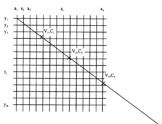
Therefore to improve the accuracy of the extrapolation for the odd very&fat cat', though more expensive in terms of computer time compared to the extrapolation procedure described earlier, the following routine is used 1. A line is constructed through the grid that intersects the origin and the point
of interest.
2. At least three evenly space points where the line passes through the grid with every increasing intervals are marked, at these points calculate the magnitude of the optimal consumption and value function, (C
i,<i) for i"1,2,l is calculated.
3. The magnitude of the value function at the point of interest is calculated by the standard bicubic interpolation/extrapolation procedure.
4. Now, we have all the information for a one-dimensional interpolation prob-lem. The consumption value of interest can be calculated by the interpolation of consumption as a function of the value function, see Fig. 3.
The algorithm describes in detail how to solve the demand side of the model. To solve the complete model requires iterating between the demand and supply sides to solve for the equilibrium set of prices. By incorporating some dampen-ing between iterations, it was possible to reduce the oscillation in the prices between iterations and consequently speed up the solution. Fig. 4 shows the convergence of the interest rate to its equilibrium value for a typical simulation.
4.3. Flexibility, robustness and speed
Fig. 3. A pictorial representation of the extrapolation algorithm.
5For comparison, Hubbard et al. (1993) discuss their solution procedure of a problem of similar complexity. They state that they needed the Cornell National Supercomputer to solve this problem because of the computational burden.
as the Euler equation, or require the problem to be reformulated in a di!erent way. Therefore, the same solution procedure can be used to solve any general consumer problem with two state variables. In theory this restriction could be relaxed too but in practice it is di$cult to see how a problem with more than three states could be solved in this way as the problem would require too much computer time.
A study of the robustness of this class of algorithms must consider two issues: the algorithm's numerical stability that is whether it will fail for any particular set of starting values, and secondly the propagation of errors through the algorithm. One of the main advantages of this procedure is that it will be very robust. Given a well-behaved utility function the optimisation problem will have no local maxima and therefore should converge globally. Secondly, as we have argued in Section 3, the errors in the calculation of the grid in any period will be increasingly attenuated in all earlier periods.
The speed of this algorithm though not fast, was certainly quick enough to make it attractive. To solve the model described in Section 2 over a simulation horizon of 100 periods where each of the 5,000 households lived for a maximum of ten periods (one period therefore represented about 7 years) took less than an hour and half on a Pentium 133 Mhz. As the model usually took around 6 to 7 iterations between the supply and demand side to converge to a tolerance of less than 1]10~3in the real interest rate, it was possible to solve a complete simulation overnight.5
5. The accuracy of the solution
an instrument set constructed from the data available in the previous period. Den Haan and Marcet (1994) show that a certain function of these correlations tends to as2distribution.
This test can be made as powerful as required in that every solution algorithm will eventually fail for a large enough sample size. This test therefore, even though it does not require a base line solution, is still comparative in nature. If the solution algorithm passes the test for a sample size say of 500 but fails it for 5000, the user has very little idea of the accuracy of his solution method. However he or she can say that it is more accurate than a solution procedure that failed the test for a sample size of 500. Its clear advantage over previous tests of accuracy is that one can infer which of two solutions is more accurate without knowing the actual solution. We will therefore propose a minor change to the use of their statistic which will allow us to something about the absolute accuracy of the solution.
As the test is based on the"rst-order conditions or Euler equations, we shall derive these"rst. To do this, it is necessary to derive an expression for the partial di!erential of the value function for three cases:"rstly if the individual died at the beginning of the period, secondly if the individual was wealth constrained and"nally for all other cases when the solution is interior. The notation is made slightly easier if we denote as<I the unconditional value function
<I
q(wq,yq)"
G
<q(wq,yq) if alive,
Bwq if died at beginning of period (6)
and so the Bellman equation (4) can be rewritten
<I
For the"rst two cases it is easy to write down the di!erential
L<I
The "rst line follows from Eq. (7) (by noting that if an individual is wealth constrained he or she will only alter their consumption in that period given slightly more or less wealth, leaving the rest of their consumption path un-altered. The second line is immediate from Eq. (6). The third case is more involved. Di!erentiating the Bellman equation (7) with respect to consumption gives the following condition for an interior solution:
and the envelope condition is simply
and substituting out for the expectation operator gives
L<I
We can therefore calculate the partial di!erential of the value function at time
tin every case. The"rst-order condition in periodt!1, given that the solution is interior, is Eq. (8) lagged by one period.
(1!d)c~t~1c"dE
t, are constructed by using the actual realised value for the partial di!erential rather than its expected value, thus
l
If the solution at time t!1 is not interior then we cannot construct an innovation for this particular consumer in this period. Equation (9) implies that these innovationsltshould be uncorrelated with any information available at time t!1. The Den Haan and Marcet (1994) simulation accuracy test is a statistical test of this observation. They suggest a test constructed from a time series of these innovations drawn from a long simulation. In their example, the system is at steady state so these innovations are drawn from a stationary stochastic process. They can therefore invoke a version of the central limit theorem due to White and Domowitz (1984) for stationary series. However in our example the distribution of the innovationltwill be a function of the age of the consumer and therefore any time series of innovations will not be stationary. We therefore suggest a slightly di!erent approach. We shall test the observation that the innovationsl
tshould be uncorrelated with any information available at timet!1 across an ensemble of simulations rather than along a time series. In this case, the Lindeberg}Feller central limit theorem is su$cient to prove the limiting results. We de"ne a set of instrumentsh
t~1made up of information
available at timet!1. For our test we chose the following
h
t~1"M1 ct~1!c6t~1 yt~1!y6t~1 wt~1!w6t~1N,
6The central limit theorem does not require the innovations to be identically distributed.
for any periodtwithin the life-span and test whether this statistic is close to zero. If we normalise the statistic by dividing through some consistent estimator of its covariance matrix which in this case is
A
t"
+
nl2tht~1h@t~1
n
then as the innovations are independently distributed6
S
t(n)"n1@2(At)~1@2BtPD N(0,I) as nPR. (10)
Den Haan and Marcet (1994) suggested the following test based on this result; calculate the single statisticS
t(n)@St(n) which should be distributed as a
s2 (4) for over 500 di!erent experiments and see what percentage of these statistics fall in the 5% tails of the s2(4) distribution. If this percentage is not too di!erent from 5% then this is evidence that the solution technique is reasonably accurate. The reason for repeating the experiment and examining the percentage falling in the tail rather than simply testing a single observation is that one e!ectively avoids the possibility of a type I error, the possibility that an accurate solution method is regarded as inaccurate. As Den Haan and Marcet (1994) note, this test can be made arbitrarily powerful by choos-ingnlarge enough. Even the most accurate solution technique will eventually fail for large enough ndue to machine round-o! error. They therefore insist that the user of the test must report the size of the sample,n, as it is an indicator of the power of the test. Campbell and Koo (1997) show that withn"1200 the test is already more discriminating than any test looking at the moment properties of the solution.
This test, as we argued earlier, is still comparative in nature. We therefore propose a minor change to the use of the statistic which is based on the strong law of large numbers. This will allow us to say something about the absolute accuracy of the solution. We shall denote our numerical estimates of the solu-tion values by a )superscript and the error between our estimate and the true value by theFsuperscript, thus
7This is the sample size used by both Den Haan and Marcet (1994) and Campbell and Koo (1997).
and using the strong law of large numbers and Eq. (10) then,
BKtP!.4. E(l8t?h
t~1)#E(l8t?hIt~1) as nPR.
If h
t~1 is exogenous then the second term on the right-hand side obviously
disappears, otherwise as long as the instruments are chosen carefully so that the error in their estimates are small the second term can be neglected as of only second order importance. Therefore the statisticB
tcan be used as a direct estimate of the absolute accuracy of the solution procedure. Thus for our example the"rst element in the row vectorB
tis simply the mean error which is c times the mean percentage error is the estimates of consumption to a
"rst order approximation. The other terms normalised by their standard errors will give a measure of any residual autocorrelation in the innova-tions.
5.1. Results of accuracy test
We carried out the accuracy test for three di!erent income processes which are now explained in order of increasing complexity (Table 2). The"rst is that an individual's income was expected to be independently and identically drawn from a log-normal distribution every period. This corresponded to parameter valueshL"h
H"0. In the second scenario an individual's income was expected
to follow a random walk with drift; this corresponded to parameter values
hL"h
H"1. The"nal scenario solved the model in its full complexity with the
following parameter values,
c r s h
L hH k p k8 p8 hI B
2 0.06 8.3 0.4 0.8 0.03 0.08 !0.31 0.3 1 10
These values include those for the income process estimated in Dutta et al. (1997). The probability of dying any period were calibrated from the UK actuary tables. In the other two scenarios all the parameter have the same values except forhL,hH.
The results of the experiment for the three di!erent income processes are recorded below. The experiment was carried out for when the grids had 10]10 and 20]20 nodes. In all experiments we use 5 point Gauss Hermite numerical integration. The den Haan and Marcet tests are reported for an ensemble size of
n"1200,7andn"5000. The accuracy statistics are calculated on an ensemble
Table 2
The results of the accuracy test
Income process Grid size den Haan}Marcet tests Accuracy test
n"1200 n"5000 E(v()/c ov,c ov,y ov,w
(%)
5% tail 95% tail 5% tail 95% tail
Complete model 10]10 4.4 5.2 3.4 8.6 !0.086 !0.002 !0.002 !0.001
20]20 4.4 4.2 5.0 5.0 0.004 0.000 0.000 !0.001
Uncorrelated 10]10 2.6 9.4 1.6 14.4 !0.132 0.006 0.007 0.001
20]20 3.8 7.8 4.2 4.8 0.009 0.001 0.001 0.000
Random walk 10]10 0.2 63.6 0.0 100.0 !0.736 0.024 0.024 !0.015
20]20 4.0 7.2 2.6 16.6 !0.043 0.004 0.004 !0.002!
!The numbers reported for the den Haan}Marcet Tests are the percentage of the 500 experiments of either 1200 or 5000 individual observations whose
statistic, given byS
t(n)@St(n), falls either below the 5th percentile or above the 95th percentile of thes2(4) distribution.
E(v()/c"+
ivi/c*100 and is an estimate of the consistent percentage error bias in the estimates of consumption across the ensemble for all individuals
aged 35.
o
v,x"+ivi(xi!x6)/J(+iv2i+i(xi!x6)2) is the autocorrelation parameter between the innovationvand the instrumentxand therefore is a measure of
any residual correlation in the innovations.
Sefton
/
Journal
of
Economic
Dynamics
&
Control
24
(2000)
1097
}
1119
8This is true except for the last few periods of the individual's life when, because of the reduced uncertainty, the solution is much more accurate.
and are expressed as coe$cient of correlation between the innovation and each of the three instruments. We have only reported the statistic for periodt"35, the mid-point of an individual's life, as those for all other periods are very similar.8
The results suggest a high degree of accuracy. The simulations for both the complete model and the i.i.d. income process pass the den Haan and Marcet test when the grid has only 10]10 nodes. The random walk model requires a"ner grid to achieve a comparable level of accuracy. In all cases there is very little correlation between the innovations and the information att!1, the major source of error seems to be a small consistent bias. This bias can be explained by the discontinuity in the di!erential of the value function due to the wealth constraint, as this discontinuity can only be approximated roughly by the polynomial splines. It will result in the solution becoming less accurate the higher the proportion of wealth constrained consumers. This explains why a higher level of resolution is required if labour income is assumed to follow a random walk with drift, because in this case a higher proportion of individuals will be wealth constrained.
6. Conclusions
In this paper we have described a numerical approach to solving the con-sumer's life-cycle problem. We have argued that the advantage of our approach is that it is versatile, and also that it is more#exible and robust than the other approaches in the literature. The method is numerically intensive but we have been able to reduce the computational burden by making e$cient use of two di!erent interpolation routines, and by calculating two interwoven grids rather than a single"ne grid. We have shown using a modi"ed den Haan and Marcet test of simulation accuracy, that the approach does achieve a high level of precision.
References
Attanasio, O., Banks, J., Meghir, C., Weber, G., 1995. Humps and bumps in lifetime consumption. Working Paper 5350, National Bureau of Economic Research.
Baxter, M., Crucini, M.J., Rouwenhorst, K.G., 1990. Solving the stochastic growth model by a discrete-state-space, Euler-equation approach. Journal of Business and Economic Statistics 8 (1), 19}21.
Campbell, J.Y., Koo, H.K., 1997. A comparison of numerical methods and analytic approximate solutions to an intertemporal consumption choice problem. Journal of Economic Dynamics and Control 21, 273}296.
Champernowne, D., 1953. A model for income distribution. Economic Journal 53, 318}351. Christiano, L.J., 1990. Solving the stochastic growth model by linear-quadratic approximation and
by value-function iteration. Journal of Business and Economic Statistics 8 (1), 23}26. Deaton, A., 1991. Saving and liquidity constraints. Econometrica 59, 1221}1248.
den Haan, W.J., Marcet, A., 1990. Solving the stochastic growth model by parameterizing expecta-tions. Journal of Business and Economic Statistics 8 (1), 31}34.
Den Haan, W.J., Marcet, A., 1994. Accuracy in simulations. Review of Economic Studies 61 (1), 3}17. Dutta, J., Sefton, J., Weale, M., 1997. Income distribution and income dynamics in the United
Kingdom. Working paper, National Institute of Economic and Social Research. Hart, P., 1976. The dynamics of earnings. Economic Journal 86, 551}565.
Hubbard, R., Skinner, J., Zeldes, S., 1993. The importance of precautionary motives in explaining individual and aggregate savings. Working Paper 4516, NBER.
Hubbard, R.G., Skinner, J., Zeldes, S.P., 1994. The importance of precautionary motives in explain-ing individual and aggregate savexplain-ing. Carnegie Rochester Conference Series on Public Policy, Vol. 40 (0), pp. 59}125.
Hubbard, R.G., Skinner, J., Zeldes, S.P., 1995. Precautionary saving and social insurance. Journal of Political Economy 103 (2), 360}399.
Keys, R., 1981. Cubic convolution interpolation for digital image processing. IEEE Transactions of Acoustics, Speech and Signal Processing 29, 1153}1161.
King, R.G., Plosser, C.I., Rebelo, S.T., 1988. Production, growth and business cycles: I. the basic neoclassical model. Journal of Monetary Economics 21 (2/3), 195}232.
Meade, J., 1976. The Just Economy. George Allen & Unwin, London.
Press, W., Teukolsky, S., Vetterling, V., Flannen, B., 1993. Numerical Recipes. Cambridge University Press, Cambridge.
Taylor, J.B., Uhlig, H., 1990. Solving nonlinear stochastic growth models: A comparison of alternative solution methods. Journal of Business and Economic Statistics 8 (1), 1}17. White, H., Domowitz, I., 1984. Non-linear regression with dependent observations. Econometrica
52, 643}661.