A novel Multiple Objective Symbiotic Organisms Search (MOSOS) for time–cost–labor utilization tradeoff problem

Contents lists available atScienceDirect

Knowledge-Based Systems

journal homepage:www.elsevier.com/locate/knosys

A novel Multiple Objective Symbiotic Organisms Search (MOSOS) for

time–cost–labor utilization tradeoff problem

Duc-Hoc Tran

a,∗

, Min-Yuan Cheng

b

, Doddy Prayogo

b,c

a_{Faculty of Project Management, University of Danang—University of Science and Technology, 54 Nguyen Luong Bang, Danang, Vietnam}

b_{Department of Civil and Construction Engineering, National Taiwan University of Science and Technology, #43, Sec. 4, Keelung Rd., Taipei 106, Taiwan} c_{Department of Civil Engineering, Petra Christian University, 121-131 Siwalankerto, Surabaya 60236, Indonesia}

a r t i c l e

i n f o

Article history:

Received 28 March 2015 Revised 21 November 2015 Accepted 24 November 2015 Available online 1 December 2015

Keywords:

Work shift Scheduling

Multi-objective analysis Symbiotic Organisms Search Time-cost-resource tradeoff

a b s t r a c t

Multiple work shifts are commonly utilized in construction projects to meet project requirements. Neverthe-less, evening and night shifts raise the risk of adverse events and thus must be used to the minimum extent feasible. Tradeoff optimization among project duration (time), project cost, and the utilization of evening and night work shifts while maintaining with all job logic and resource availability constraints is necessary to enhance overall construction project success. In this study, a novel approach called “Multiple Objective Sym-biotic Organisms Search” (MOSOS) to solve multiple work shifts problem is introduced. The MOSOS algorithm is new meta-heuristic based multi-objective optimization techniques inspired by the symbiotic interaction strategies that organisms use to survive in the ecosystem. A numerical case study of construction projects were studied and the performance of MOSOS is evaluated in comparison with other widely used algorithms which includes non-dominated sorting genetic algorithm II (NSGA-II), the multiple objective particle swarm optimization (MOPSO), the multiple objective differential evolution (MODE), and the multiple objective ar-tificial bee colony (MOABC). The numerical results demonstrate MOSOS approach is a powerful search and optimization technique in finding optimization of work shift schedules that is it can assist project managers in selecting appropriate plan for project.

© 2015 Elsevier B.V. All rights reserved.

1. Introduction

Labor is a critical construction project resource for construction contractors to be successful on every construction project. Inefficient management of labor resources can result the contractors not able to meet the project deadline and budget requirement. When facing a tight schedule deadline, labor resources has a huge limitation on the number of hours a worker can work per day. Therefore, it requires the use of shift work to meet scheduled deadlines[1]. Using shift work can approximately double the total amount of work hours per day. It also has an advantage over using overtime hours because it prevents worker fatigue and has lower hourly labor costs[2,3]. Furthermore, work shift done during the evening and night is often more efficient due to the quieter, less congested environment around the construc-tion site.

In spite of these advantages, the multiple shift schedules possess several shortcomings including its negative impacts on construction cost, productivity, and safety[1,4]. The multiple shifts might lead in

∗ _{Corresponding author. Tel.: +84 988922999.}

E-mail addresses:tdhoc@dut.udn.vn,duchoc87@gmail.com(D.-H. Tran), myc@mail.ntust.edu.tw(M.-Y. Cheng),doddyprayogo@ymail.com(D. Prayogo).

higher overall costs that are required for shift premiums, quality con-trol, nighttime lighting, and safety measures. Additionally, disturbed sleep cycles and stress resulting in higher injury and accident risks, and nighttime construction adversely affects worker health due to circadian rhythm disruption[5–7]. Moreover, recent researches iden-tified that the utilization of evening and night shifts causes higher rates of labor overturn and absenteeism that leads to project delays and cost overruns[2,4]. In order to minimize these negative impacts of utilizing multiple shifts while complying with labor availability constraints, project decision makers need to distribute and utilize the limited labor resources among multiple shifts in the most efficient and effective way to maximize project performance.

Over past decades, a significant amount of research studies have developed optimization models to solve civil engineering problems ranging from structural engineering[8]to construction management [9]. In recent years, there have been notable efforts to solve resource utilization problems using multi-objective optimization models. The most commonly used multi-objective optimization model is the mul-tiple objective genetic algorithm (GA)[10–13]. Other researchers have developed hybrid models of genetic and other algorithms such as par-ticle swarm optimization (PSO)[14], differential evolution (DE)[15] and simulated annealing[16]. However, there are a few reported re-searches that focus on optimizing the utilization of multiple labor

D.-H. Tran et al. / Knowledge-Based Systems 94 (2016) 132–145 133

shifts in constructions. Jun and El-Rayes[1]firstly applied a multi-ple objective genetic algorithm to work shift problem. Therefore, fur-ther study is needed to build better optimization models to schedule construction project work shift.

Symbiotic Organisms Search (SOS) is currently one of the most recent metaheuristic algorithms[17]. SOS was first used in a wide va-riety of highly nonlinear benchmark and engineering problems. The SOS algorithm is simply structured and easy to use, while demon-strating great robustness and fast convergence in solving single ob-jective global optimization problem. Preliminary studies indicate that the new SOS algorithm is superior over the widely used GA, PSO, DE, and bees algorithm (BA) in solving a various continuous benchmark function and engineering problems[17]. Since the SOS algorithm is relatively new, the capability of the SOS algorithm in solving the time cost utilization labor tradeoff (TCUT) problem is very interesting to be further explored and investigated.

This study presents the novel Multiple Objective Symbiotic Or-ganisms Search (MOSOS) algorithm to facilitate a TCUT analysis. The important contribution of this research is that the proposed MOSOS algorithm is a new, multiple objective optimization (MOO) version of the basic SOS algorithm. MOSOS algorithm is developed to fit the TCUT problem because the ability to provide efficient solutions for complex problems simpler operations of SOS is very much attractive and encouraging. The proposed algorithm is designed to attain fast convergence without losing solution diversity on the Pareto front.

The remaining of this paper is organized as follows. InSection 2, the time-cost-utilization resource problem is mathematically formu-lated. InSection 3, literature related to the establishment of the new optimization model is briefly reviewed. InSection 4, the detailed de-scriptions of the proposed optimization model for the TCUT problem are presented in details. InSection 5, the performance of the newly developed model is demonstrated using two numerical experiments and result comparisons.Section 6presents study conclusions. 2. Work shift schedules problem formulation

Using multiple work shifts in a construction project requires that the project planners determine the execution mode of project activi-ties, seek to find the optimal scheduling sequence and assign workers to shifts while satisfying all project constraints. The work shift prob-lem must minimize three contradicting objectives simultaneously in-cluding project duration, project cost, and total evening and night shift working hours[1].

The first objective, minimization of total project duration, may be expressed as follows:

Minimize project time T=

l

n=1

TSn

n =Max∀n

(

ESn+Dn

)

ESn= Maximum

all predecessorsmofn

(

ESm+Dm

)

(1)

whereTSn

n is the duration of the activityn

{

n=1,2, . . . ,l

}

on the

criti-cal path for a specific option of resources (Sn);lis the total number of

critical activities on a specific critical path.ESnis the earliest start of

activityn, Dnis the duration of activityn. In general, project duration

is calculated based on precedence constraints and activity duration. The project information determines the precedence constraints and the selection alternatives determine activity duration.

The second objective, minimization of total project cost, may be calculated as follows:

Minimize projectcost=

N

i=1

CostSi

i (2)

whereCostSi

i is the total cost which includes direct and indirect cost

of activityifor a specific option of resources (Sn) andNis the total

number of activities.

The third and final objective, minimization of project labor utiliza-tion in evening and night shifts, may be calculated as follows.

Minimize LHEN=LHE+LHN

(

1+W

)

if SS

=3

(

Three shifts system

(

SS

))

(3)

LHNE=LHE if SS=2

(

Two shifts system

)

(4)

LHE=

N

n=1

(

Dn∗Rn,2

)

∗HE (5)

LHN=

N

n=1

(

Dn∗Rn,3

)

∗HN (6)

whereLHEN is the total number of evening and night shift work hours,LHEis the total number of evening shift work hours andLHN is the total number of night shift work hours. Because risks faced in night shift work are typically higher than in other shifts,Wis the de-fined weight that represents the relative importance of minimizing LHN. Rn, kis the daily labor demand of activitynon shiftk. k

repre-sents the shift type (e.g., for the 3-shift system,k=1 means day shift, k=2 means evening shift, andk=3 means night shift);HEis the daily evening shift work hours (7.5 h per day); andHNis the daily night shift work hours (7 h per day). In this study, day shift is the pe-riod of time for such work during the day (as 8 a.m. to 4 p.m. – 8 h). Evening shift is the work shift during the evening (as 4 p.m. to mid-night). Night shift is the work shift during the night (as midnight to 8 a.m.).

3. Literature review

3.1. Review of multiple objective optimization

A MOO problem involves several conflicting objectives simultane-ously. The MOO with such conflicting objective functions gives rise to a set of Pareto optimal solutions instead of one optimal solution. Because no one of these solutions can be considered to be better than any other with respect to all objective functions. Generally, the MOO problem consists ofndecision variables,kobjective functions,m in-equality constraints andpequality constraints. It may be mathemat-ically formulated as follows[18–20]:

min

X∈D f

(

X

)

=[f1

(

X

)

,f2

(

X

)

, . . . ,fk

(

X

)

] (7)

s.tgi

(

X

)

≥0; i=1, . . . ,m (8)

hj

(

X

)

=0; j=1, . . . ,p (9)

D=

{

X

|

g

(

X

)

≥0,h

(

X

)

=0

}

(10)

wheref(X)is the objective vector,kis the number of objective func-tions.gi(X) is the set of inequality constraints, andhj(X) is the set of

equality constraints. The solutionX

(

x1,x2, . . . ,xn

)

T is a vector ofn

decision variables in feasible regionD. The multi-objective optimiza-tion problem works to determine those vectorsXthat yield the opti-mum values for all the objective functions from the setDof all vectors which satisfy (8) and (9).

Because this problem rarely presents a unique solution, decision makers are expected to choose a solution from among a set of effi-cient solutions, known collectively as the Pareto. The Pareto domi-nance is formally defined as follows (Deb[18]):

SolutionX1

(

x1.1,x1.2, . . . ,x1.n

)

TdominatesX2

(

x2.1,x2.2, . . . ,x2.n

)

T

if both the conditions are satisfied:

1.

∀

i∈

(

1,2, . . . ,k

)

: f_i

(

X1

)

≤ fi

(

X2

)

. The solutionX1is no worse

thanX2in attaining all objectives.

2.

∃

i∈

(

1,2, . . . ,k

)

:fi

(

X1

)

<fi

(

X2

)

. The solutionX1 is strictly

So, while comparing two different solutionsX1andX2, there are

three possibilities of dominance relation between them.

• X₁dominatesX₂ • X1is dominated byX2

• X₁andX₂are non-dominated to each other.

A non-dominated solution means that no other solution has been found that dominates it. The set of non-dominated solutions is called the Pareto front.

Multiple Objective Evolutionary Algorithms (MOEAs) have at-tracted increasing attention for solving MOO problems[21–24]in re-cent years. Various researchers from various multi-disciplinary have used MOEAs to solve optimization problems that arise in their own fields[25–27]. As MOO problems become more complex, new MOEAs will continue to emerge.

3.2. Symbiotic Organisms Search algorithm

The SOS algorithm is a new meta-heuristic algorithm devel-oped by Cheng and Prayogo [17]. It is inspired by the biological dependency-based interaction seen among organisms in nature. The dependency-based interaction is often known as symbiosis. Like most population-based meta-heuristic algorithms, SOS shares the similar following features: it uses a population of organisms which contains candidate solutions to seek the global solution over the search space; it has special operators that employ the candidate solutions to guide the searching process; it uses a selection mecha-nism to preserve the better solutions; it requires a proper setting of common control parameters such as population size and maximum number of evaluations.

However, unlike most meta-heuristic algorithms which have ad-ditional control parameters (i.e. GA has crossover and mutation rate; PSO has inertia weight, cognitive factor, and social factor), SOS re-quires no algorithm-specific parameters. This is considered as an advantage over competing algorithms since SOS does not need ad-ditional work for tune the parameters. Improper tuning related to the algorithm-specific parameters might increase the computational time and produce the local optima solution.

In the early stage, a random ecosystem (population) matrix is created, each row representing a candidate solution to the corre-sponding problem. The number of organisms in the ecosystem, so-called the ecosystem size, is pre-determined by the users. The rows in the matrix are called organisms, same as individuals in other meta-heuristic algorithms. Each virtual organism represents a candidate solution to the corresponding problem/objective. The search begins after the initial ecosystem generated. During the searching process, each organism gains benefit from continuously interacting with one another through three different ways:

1. Mutualism phase: The phase where one organism is develop-ing a relationship that benefits itself and also the other. The interaction between bees and flowers is a classic example to explain the philosophy of mutualism.

2. Commensalism phase: The phase where one organism is de-veloping a relationship that benefits itself while does not im-pact the other. An example of commensalism is the relation-ship between remora fish and sharks.

3. Parasitism phase: The phase where one organism is develop-ing a relationship that benefits itself but harms the other. An example of parasitism is the plasmodium parasite, which uses its relationship with the anopheles mosquito to pass between human hosts.

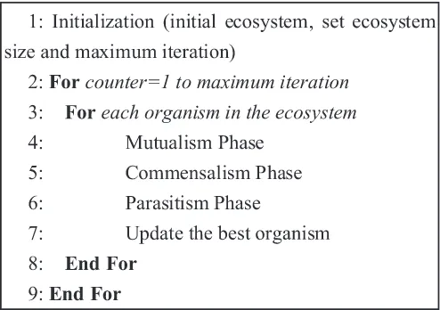
These three phases are adopted from the most common sym-bioses used by organisms to increase their fitness and survival advan-tage over the long term. During the interaction, the one who receive a benefit will evolve to a fitter organism while the one who is harmed

Fig. 1. SOS algorithm pseudocode.

will perish. The mechanisms for updating the best organism will be conducted after one organism has completed their three phases. The phase will operate until the stopping criterion is achieved. The pseu-docode shown inFig. 1further summarizes the basic step SOS opti-mization procedure.

4. The proposed Multiple Objective Symbiotic Organisms Search for time–cost–utilization labor tradeoff model (MOSOS-TCU)

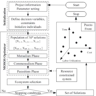
This section describes the Multiple Objective Symbiotic Organ-isms Search (MOSOS) for solving the TCUT problem developed in this study based on the original SOS algorithm[17].Fig. 2shows the over-all operational architecture of the proposed algorithm. The following subsections provide further details on the flowchart.

4.1. Ecosystem initialization

This study considers the TCUT problem, in which project cost, project duration, and the utilization of evening and night work shifts are optimized simultaneously. The model requires project informa-tion inputs including activity relainforma-tionship, activity durainforma-tion (Duri),

activity cost (Ci), daily labor demand (Ri,j), shift options (Si) for each

activity, and total number of available labor (RC). In addition, the user also must provide parameter settings for the search engine (MOSOS) such as the value of ecosystem sizeecosize, number of decision vari-ablesD, number of objective functionsM, maximum number of gen-erationsGmax, the lower bound (LB) and the upper bound (UB) of

deci-sion variables. With these inputs, the optimizer conducts calculations to obtain an optimal set of shift options, optimal scheduling sequence and assign available labors to shifts for all construction project activ-ities. With all the necessary information provided, the model is capa-ble of operating automatically without any human intervention.

Population (ecosystem) initialization is the first and the primary task in any optimization algorithm. These two terms, population and ecosystem or, are used interchangeably. Analogous to other population-based algorithms, MOSOS begins with an initial popula-tion called the ecosystem. In the initial ecosystem, a group of organ-isms is generated randomly to the search space as follows:

The initial process generates a point inD-dimensional spaceX=

{

x1,x2, . . . ,xD

}

in whichx1,x2, . . . ,xD∈ ℜandxj∈[0, 1] have uniform

random distributions. The firstecosizeorganisms may be easily gen-erated as follows:

X_i,jG=0=LBj+xi,j∗

(

UBj−LBj

)

;i=1,2, . . . ,D;

D.-H. Tran et al. / Knowledge-Based Systems 94 (2016) 132–145 135

Fig. 2.MOSOS for the TCUT problem flowchart.

4.2. Decision variables and constraints

A candidate solution to the TCUT problems may be represented as a vector with these decision variables: (1) shift option used for each activity; (2) the priority value of each activity; and (3) the labor con-straint with (2N+ 1), (2N+ 2) elements for two, three shifts system, respectively, as follows:

X=

⎡

⎢

⎣

xi,1, . . . ,xi,j, . . . ,xi,N

Shift−OptionSn

,xi,N+1, . . . ,xi,2N

Priority−valuePn

, xi,2N+1,xi,D

Labor−ConstraintLk/RC

⎤

⎥

⎦

(12)

whereDis the number of decision variables in the problem at hand. It is obvious thatNis the number of activities in the project network. Indexidenotes theith individual in the population.

(1) Shift option: Shift-option (Sn) represents the feasible shift

op-tions for activityn. Every option has specific combinations of duration, cost and labor demands that lead to different total project durations, total costs and total labor hours. Vectorxi,n

represents one shift option value for activityn. Si,nis an

inte-ger number in the range [1,USn] (n=1 toN), meaning one

po-sition fromUSnshift options. Because the original DE operates

with real-value variables, a function is employed to convert the execution mode options of those activities from real values to integer values within the feasible domain.

Si,n=Round

(

xi,n×USn

)

;

(

n=1, . . . ,N

)

(13)

wherexi, nis the shift option value of activitynat the individual ith.USnrepresents the total number of shift options for each

activity. Round is a function to convert a real number to the nearest integer greater than or equal to it.

(2) Priority value: priority-value (Pn) represents the preference

value for each activity in comparison with all other activities. Eq. (14)shows the constraint for this variable.

0≤Pn≤1; n=N, . . . ,2N (14)

Together with labor constraints and the precedence relation-ships between activities,Pnvalues help determine the project

scheduling sequence and calculate project duration based the resource constraint subsystem presented in the following sub-section.

(3) Labor constraints: labor-constraint (Lk/RC) represents the

per-centage of total available labors per day for shiftk.Eq. (15) shows the constraint for this variable.

0≤Lk/RC≤1; k=1,K−1 (15)

whereRCis the total number of labors per day available for distribu-tion among all shifts;kis shift type; andKis the maximum number of allowable shifts per day (e.g.K=3 for three shifts andK=2 for two shifts). This decision variable limits the amount of workers per shift and determines the allocation of available workers. The labor availability (RCSk) for each shift in the three-shift system may be

cal-culated as follows:

MRk=max

n∈All

{

R Sn

n,k

}

(16)

REM=RC−K

k=1MRk (17)

PR1=Round

(

REM∗

(

L1/RC

))

(18)

PR2=Round

(

REM−PR1

)

∗

(

L2/RC

)

(19)

RCS1=MR1+PR1 (20)

Fig. 3.Transfer to feasible active schedule.

RCS3=RC−

(

RCS1+RCS2

)

(22)

whereMRkis the minimum number of workers for shiftk; REMis the

remaining number of available workers;PR1is the additional number

of workers available for allocation to the day shift;PR2is the

addi-tional number of workers available for allocation to the evening shift; RCS1is the maximum number of workers allowed to be allocated to

the day shift;RCS2is the maximum number of workers allowed to be

allocated to the evening shift; andRCS3is the maximum number of

workers allowed to be allocated to the night shift.

4.3. Resource constraint subsystem

Once the MOSOS organism is created, the project duration is cal-culated through serial method. The shift-option (Sn) values of MOSOS

organism defines the execution mode of each activity and then deter-mines the corresponding durations and resource requirements of all activities. The priority value (Pn) of MOSOS organism carries out the

sequence of activities. Labor-constraint (Lk) figure out the number of

available labors per day for each shift.

The serial method was proposed by Kolisch [28]. It consists of n=1,…,Nstages, in which one activity is selected and scheduled in each stage. When an activity has been checked and currently avail-able amounts of resources are adequate, this activity is scheduled at the earliest precedence time (e.g., the earliest completion times of its predecessors) and resource-feasible time. The serial schedule schema is revised for easier comprehension and implementation using the following two steps:

Step 1: Transfer MOSOS organism sequence of tasks priorities to an active schedule based on precedence constraints.

Denote a set of tasks in project J=

{

1,2, . . . ,N

}

. We can define priority relations in setJas a set of pairC=

{

(

i,j

)

|

ithat must be exe-cuted beforej}. We introduce the binary relation matrixV=

(

v

_{i j,}1_≤

i,j≤n

)

,

v

_{i j}=1, if (i, j)∈C,

v

_{i j}=0, if (i, j) ∈C, related with a set of prior-ity constraints and define a full-priorprior-ity relation matrixG=

(

gi j,1≤ i,j≤n

)

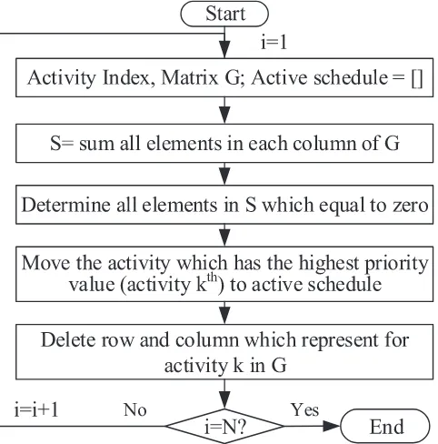
. This matrix describes all priority relation chains. So,g_{k j}=1 if it is possible to find such a sequence of index pairs that (k, k1)∈

C, (k1,k2)∈C,…,(kl, kj)∈C. The matrix V has the following property:

v

_{i j=}1_⇒

v

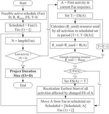
_ji=1. The G matrix shares this feature as well[29].Fig 3 illustrates the transfer procedure.

Step 2: Calculate project duration based on active schedule Two important points must be considered before applying the serial method. Firstly, activity A starts when all predecessors are completed (network logic). Secondly, activity A start time depends on resource availability. Thus, activity A is scheduled to start after the completion time of its immediate predecessor on the histogram at the point when sufficient resources are available for activity comple-tion (resource constrained).Fig 4demonstrates how the serial gener-ation calculates project durgener-ation.

The search engine (MOSOS) takes into account the results ob-tained from the scheduling module and the search for an optimal combination of shift work options, optimal scheduling sequence for each activity and assign available labors to shifts. This research used three contradicting objectives.Section 2describes the formulae for each objective function.

4.4. Mutualism phase

LetXibe the organism matched to theith row of the ecosystem

population. The organismXiselects organismXjas its partner

ran-domly from the ecosystem. OrganismXiis associated to thejth row

of the ecosystem wherejis different fromi. The mutualistic symbiosis between organismXiandXjis modeled inEqs. (23)and(24).

Xinew=Xi+rand

(

0,1

)

∗

(

Xbest−Mutual_Vector∗BF1

)

(23)

Xjnew=Xj+rand

(

0,1

)

∗

(

Xbest−Mutual_Vector∗BF2

)

(24)

Mutual_Vector= Xi+Xj

2 (25)

Some notes on the mutualism mathematical model:

1. rand(0,1) inEqs. (23)and(24)is a vector of random numbers between 0 and 1.

2. “Mutual_Vector” represents the mutual connection between organismX_iandX_j.

3. Xbest represents the best organism in an ecosystem. In this

model, the Xbest is arbitrarily chosen among the first

non-dominated rank.

4. OrganismXimight benefit significantly when interacting with

organismXj. Meanwhile, organismXjmight only get benefit

slightly when interacting with organismXi. Here, Benefit

Fac-tors (BF1) and (BF2) are determined stochastically as either 1

or 2. This illustrates whether an organism partially or fully benefits from the interaction.

5. Organisms are evolving to a fitter version only if their new fit-ness dominates their pre-interaction fitfit-ness. In this case, the oldXiandXjwill be replaced immediately byXi newandXj new,

respectively. The oldX_iandX_jwill be moved into advanced population. Otherwise, theXi newandXj newwill be added into

advanced population for selecting the next generation ecosys-tem. In this way, the proposed algorithm can converge faster while maintaining good diversity. Since algorithm may gain some important information from dominated the solution in latter sorting.

6. For each organismXi, this interaction counts for two function

evaluations.

4.5. Commensalism phase

After the mutualism phase is finished, the organism Xi selects

again a new partner randomly from the ecosystem, organismX_j. In this circumstance, organismXiattempts to benefit from the

interac-tion but organismXjneither benefits nor suffers from the

relation-ship. The commensal symbiosis between organismXiandXjis

mod-eled inEq. (26).

D.-H. Tran et al. / Knowledge-Based Systems 94 (2016) 132–145 137

Fig. 4. Serial method.

Some notes on the commensalism mathematical model:

1. rand(−1,1) inEq. (26)is a vector of random numbers between −1 and 1.

2. Xbest reflects the best organism in the ecosystem, similar to

those in the mutualism phase.

3. OrganismXiis updated byXi new only if its new fitness

dom-inates its pre-interaction fitness. Then,Xiwill be moved into

advanced population, otherwise,Xi new. This selection

mecha-nism is analogous to those in the mutualism phase.

4. For each organismXi, this interaction counts for one function

evaluation.

4.6. Parasitism phase

After the commensalism phase is completed, the organismX_i se-lects again a new organism randomly from the ecosystem, organism Xj. In parasitism, organismXiis given a role similar to the

anophe-les mosquito through the creation of an artificial parasite called “Par-asite_Vector”. OrganismXj serves as a host to the Parasite_Vector.

During the interaction, theParasite_Vectortries to kill the hostXjand

replaceXjin the ecosystem. The organismXimay gain a benefit,

be-cause by cloning it, its influence in the ecosystem may increase while Xjmay have to suffer and die.

The creation ofParasite_Vectoris described as follows:

1. InitialParasite_Vectoris created in the search space by dupli-cating organismXi. Some decision variables from the initial

Parasite_Vectorwill be modified randomly in order to differ-entiateParasite_Vectorwith organismXi.

2. A random number is created within a range from one to the number of decision variables. This random number represents the total number of modified variables.

3. The location of the modified variables is determined stochastically.

4. Finally, the variables are modified using a uniform distribu-tion within the range of the search space. TheParasite_Vector is ready for the parasitism phase.

BothParasite_Vectorand organismXjare then evaluated to

mea-sure their fitness. IfParasite_Vectordominates or non-dominated each other withX_j, it will replace organismX_jin the current ecosystem andXjwill be moved into advanced population. Otherwise, the Para-site_Vectorwill be moved into advanced population. For each organ-ismX_i, this interaction counts for one function evaluation.

4.7. Ecosystem selection procedure

Fig. 5. Ecosystem selection procedure.

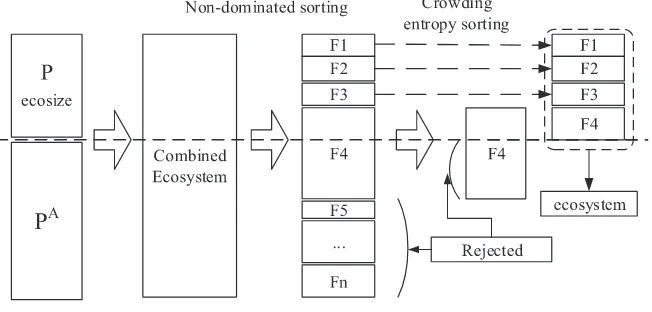
in the single objective solution scenario, a two-solution dominance approach is used in multi-objective scenarios. Note that the total size of the combined population is larger thanecosize. However, popula-tion size during the optimizapopula-tion process remainsecosize. Thus, eco-sizesolutions are selected based on the technique as follow. At first, thus, the fast non-dominated sorting technique[31]is employed to sort the combined population into non-dominated sets (F1,F2, …).

The solutions belonging to the best non-dominated set (SetF1) are

se-lected first to enter the main population. If size ofF1is smaller than

ecosize, the remaining members of the population are chosen from subsequent non-dominated fronts in rank order (F2,F3…). This

pro-cedure continues until no further sets can be accommodated. Assume thatFkis the last non-dominated set beyond which no other set can

be accommodated. In general, the number of solutions in all setsF1

toF_kis greater thanecosize. To select the optimalecosizepopulation members using crowding entropy sorting technique[32], it is neces-sary to first fill all population slots in descending order of distance. Fig 5provides an overview of this procedure.

4.8. Stopping conditions

The optimization process terminates when the stopping condi-tions are achieved. The user can set these types of condicondi-tions. Maxi-mum generationGmaxor maximum number of functions evaluations

(NFE) may be used as the stopping criterion. This study used the max-imum number of generation as stopping condition for the proposed algorithm. When the optimization process ends, the final set of op-timal solutions, called the Pareto front, is presented to the user. Ob-taining the entire Pareto front is of great importance because it as-sists planners to evaluate the pros and cons of each potential solution based on qualitative and experience-driven considerations.

5. Case study

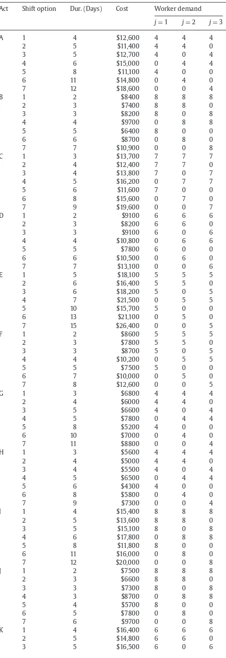
This study analyzed a numerical case to demonstrate the effec-tiveness of the proposed MOSOS for the TCUT problem, with obtained results compared against four approaches also employed to handle the TCUT problem, including NSGA-II, MOPSO, MODE and MOABC. The case project adapted was a previous study of a construction project by Jun and El-Rayes[1]. The project comprised 15 construc-tion activities, each of which has a number of possible shift alterna-tives. In the case study, a three shifts system (SS=3) was utilized in combination with a total of 70 available daily labors (RC=70). The weight for night shift inEq. (3)was set asW=80%.Fig. 6shows the precedence relationships of the network projects.Table 1illustrates project information data including allowable types of shift operation for each activity (n) and its direct cost, duration, and daily labor de-mand for each shift and Shift-option (Sn) for project. Project with an

average of seven execution modes for each of the 15 activities gener-ate multiple billions 715_{of possible combinations for completing the}

entire projects. Each possible combination has a unique impact on project performance, which means that DMs must search in a large number of potential solutions to find those that establish an optimal tradeoff/balance among construction duration, cost, and the utiliza-tion of evening and night work shifts. The newly developed multi-objective optimization model was used to search the many potential solutions.

5.1. Optimization result of MOSOS-TCUT

Since the original SOS is the core mechanism in the proposed MOSOS-TCUT. Only two common control parameters which are pop-ulation size and maximum number of generations are needed to be

D.-H. Tran et al. / Knowledge-Based Systems 94 (2016) 132–145 139

Table 1

Case study data.

Act Shift option Dur. (Days) Cost Worker demand

j=1 j=2 j=3

A 1 4 $12,600 4 4 4

2 5 $11,400 4 4 0

3 5 $12,700 4 0 4

4 6 $15,000 0 4 4

5 8 $11,100 4 0 0

6 11 $14,800 0 4 0

7 12 $18,600 0 0 4

B 1 2 $8400 8 8 8

2 3 $7400 8 8 0

3 3 $8200 8 0 8

4 4 $9700 0 8 8

5 5 $6400 8 0 0

6 6 $8700 0 8 0

7 7 $10,900 0 0 8

C 1 3 $13,700 7 7 7

2 4 $12,400 7 7 0

3 4 $13,800 7 0 7

4 5 $16,200 0 7 7

5 6 $11,600 7 0 0

6 8 $15,600 0 7 0

7 9 $19,600 0 0 7

D 1 2 $9100 6 6 6

2 3 $8200 6 6 0

3 3 $9100 6 0 6

4 4 $10,800 0 6 6

5 5 $7800 6 0 0

6 6 $10,500 0 6 0

7 7 $13,100 0 0 6

E 1 5 $18,100 5 5 5

2 6 $16,400 5 5 0

3 6 $18,200 5 0 5

4 7 $21,500 0 5 5

5 10 $15,700 5 0 0

6 13 $21,100 0 5 0

7 15 $26,400 0 0 5

F 1 2 $8600 5 5 5

2 3 $7800 5 5 0

3 3 $8700 5 0 5

4 4 $10,200 0 5 5

5 5 $7500 5 0 0

6 7 $10,000 0 5 0

7 8 $12,600 0 0 5

G 1 3 $6800 4 4 4

2 4 $6000 4 4 0

3 5 $6600 4 0 4

4 5 $7800 0 4 4

5 8 $5200 4 0 0

6 10 $7000 0 4 0

7 11 $8800 0 0 4

H 1 3 $5600 4 4 4

2 4 $5000 4 4 0

3 4 $5500 4 0 4

4 5 $6500 0 4 4

5 6 $4300 4 0 0

6 8 $5800 0 4 0

7 9 $7300 0 0 4

I 1 4 $15,400 8 8 8

2 5 $13,600 8 8 0

3 5 $15,100 8 0 8

4 6 $17,800 0 8 8

5 8 $11,800 8 0 0

6 11 $16,000 0 8 0

7 12 $20,000 0 0 8

J 1 2 $7500 8 8 8

2 3 $6600 8 8 0

3 3 $7300 8 0 8

4 3 $8700 0 8 8

5 4 $5700 8 0 0

6 5 $7800 0 8 0

7 6 $9700 0 0 8

K 1 4 $16,400 6 6 6

2 5 $14,800 6 6 0

3 5 $16,500 6 0 6

Table 1(continued)

Act Shift option Dur. (Days) Cost Worker demand

j=1 j=2 j=3

4 6 $19,400 0 6 6

5 8 $14,000 6 0 0

6 11 $18,800 0 6 0

7 12 $23,600 0 0 6

L 1 1 $6100 8 8 8

2 2 $5500 8 8 0

3 2 $6100 8 0 8

4 2 $7200 0 8 8

5 3 $5100 8 0 0

6 4 $6900 0 8 0

7 4 $8600 0 0 8

M 1 2 $3300 3 3 3

2 3 $2900 3 3 0

3 3 $3300 3 0 3

4 4 $3900 0 3 3

5 5 $2500 3 0 0

6 6 $3500 0 3 0

7 7 $4300 0 0 3

N 1 4 $13,400 7 7 7

2 5 $11,900 7 7 0

3 5 $13,200 7 0 7

4 6 $15,600 0 7 7

5 8 $10,300 7 0 0

6 11 $14,000 0 7 0

7 12 $17,500 0 0 7

O 1 2 $7700 8 8 8

2 3 $6800 8 8 0

3 3 $7500 8 0 8

4 3 $8900 0 8 8

5 4 $5900 8 0 0

6 6 $8000 0 8 0

7 6 $10,000 0 0 8

Note: shift optionSn=1: three shifts (day, evening, and night shifts),Sn=2: two shifts (day and evening shifts),Sn=3: two shifts (day and night shifts),Sn=4: two shifts (evening and night shifts),Sn=5: one shift (day shift),Sn=6: one shift (evening shift),Sn=7: one shift (night shift).

Table 2

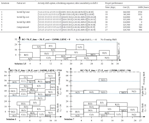
Best non-dominated solutions obtained by MOSOS-TCUT.

Solutions Partial set Activity shift-option, scheduling sequence, labor availability in shiftk Project performance

Time (days) Cost ($) LHEN (hours)

1 Sorted by time {1.2.1.2.1.5.1.2.2.5.1.5.1.1.1}{A.B.F.C.D.E.G.H.J.I.K.L.M.N.O}{32.20.18} 18 144,500 3710 2 {1.2.1.2.2.5.1.2.2.5.1.5.1.2.1}{A.B.F.C.D.E.G.H.J.I.K.L.N.M.O}{32.20.18} 19 141,300 3132 3 Sorted by cost {5.5.5.5.5.5.5.5.5.5.5.5.5.5.5}{A.B.F.C.D.E.J.G.H.I.K.L.M.N.O}{30.20.20} 38 124,900 0 4 {2.5.5.5.5.5.5.5.5.5.5.5.5.5.5}{A.B.C.D.E.F.J.G.H.I.K.L.M.N.O}{32.26.12} 35 125,200 150 5 Sorted by LHEN {5.5.5.5.5.5.5.5.5.5.5.5.5.5.5}{A.B.F.C.D.E.J.G.H.I.K.L.M.N.O}{30.20.20} 38 124,900 0 6 {5.5.5.5.5.5.2.5.5.5.5.5.5.5.5}{A.B.F.C.D.E.J.G.H.I.K.L.M.N.O}{38.14.18} 35 125,700 120 7 Compromised {2.5.5.5.2.5.1.5.5.5.5.5.2.2.5}{A.B.C.D.E.F.J.G.H.I.K.L.M.N.O}{36.19.15} 27 129,500 946 8 {2.5.2.5.2.5.2.5.5.5.2.5.2.5.5}{A.B.C.D.E.F.G.H.J.I.K.L.M.N.O}{35.16.19} 27 128,700 998

Fig. 7. Schedules related to three non-dominated solutions of case study.

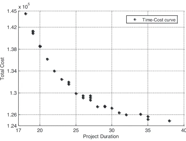
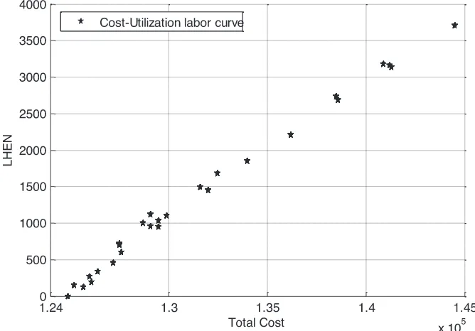
Figs. 8–10 show the two objectives relationship between time and cost, cost and labor utilization, and time and labor utilization, respectively, on a two-dimensional plane. It can be seen from the time-cost curve example (Fig. 9) that lower project funding cor-relates with longer project completion duration and vice versa. Nevertheless,Figs. 8–10 might not be good representatives of the entire tradeoff surface in the three-dimensional space. In fact, the two-dimensional tradeoff surface, when projected from three to two dimensions, might lose some non-dominated points because there is a hidden dimension that makes these points non-dominated.

5.2. Statistical comparison and analysis

We compared MOSOS performance against NSGA-II[31], MOPSO [34], MODE[30]and MOABC[35]to assess comparative effectiveness. For comparison purposes, all five algorithms used an equal number of function evaluations, had a population size of 200 and a maximum of 300 generations. In NSGA-II, the constant mutant and crossover prob-ability factors were set at 0.5 and 0.9, respectively. In MOPSO, the two learning factorsc1,c2are both chosen at 2, and the inertia factorwis

set in range of 0.3–0.7. In MODE, the crossover probability CR is set to 0.8, and the scaling factorFequals to 0.5. MOSOS control parameters

remained the same as stated in previous subsection. Thirty indepen-dent runs were carried out for all experiments in case study.

Much research effort has been invested in recent years to de-velop methods able to evaluate the performance of multi-objective optimization models. Its complex characteristics mean that multi-objective optimization results cannot be evaluated directly, unlike those of single-objective optimization. In the literature, the re-searchers have suggested numerous quality indicators [31,36–38]. This study used the following four evaluation methods.

1. Number of solutions found in the Pareto-optimal front: the goal of multi-objective optimization is to obtain the Pareto-optimal front that contains the non-dominated solutions of the problem under investigation. No single solution in the Pareto-optimal front may be objectively evaluated as being better than its peers[39]. Therefore, it is preferable to find as many solutions within the Pareto-optimal front as possible. Table 3shows that MOSOS earned the highest number of so-lutions found in the Pareto front evaluation criterion with 20.9 solutions on average.

D.-H. Tran et al. / Knowledge-Based Systems 94 (2016) 132–145 141

Fig. 8.Time–cost–utilization labor tradeoff Pareto front using MOSOS.

Fig. 9. Time–cost tradeoff curve.

two sets of decision solutions. C-metric is defined as the map-ping between the ordered pair (S1,S2) and the interval [0,1]:

C

(

S1,S2

)

=

|{

a2∈S2;

∃

a1∈S1:a1≤a2

}|

|

S2

|

(24)

The numerator inEq. (24)denotes that the number of solutions inS2is dominated by at least one solution inS1, the

denomi-nator is the total solutions inS2. Provided thatC(S1,S2)=1,

all solutions inS2 are dominated by or equal to solutions in

S1. IfC(S1,S2)=0, thenS1covers none of the solutions inS2.

BothC(S1,S2) andC(S2,S1) should be checked in the

compari-son because C-metric is not symmetrical in its arguments[41]. Table 4illustrates comparison results among four algorithms in terms of C-metric, where A1, A2, A3, A4 and A5 indicate

MOSOS, MODE, MOABC, MOPSO, and NSGA-II, respectively. Re-sults show that MOSOS dominates more than 67.2% of MODE solutions, 94.4% of MODE solutions, 100.0% of MOPSO solu-tions, and 100.0% of NSGA-II solutions on average.

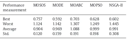
3. Spread (SP): this indicator[32]measures the extent of spread achieved among the non-dominated solutions. The mathemat-ical definition of SP may be given as:

SP=

k

i=1d

(

Ei,

)

+X∈

d

(

X,

)

−d

k

i=1d

(

Ei,

)

+

(

|

|

−k

)

d

(25)

where

is a set of solutions,

(

E1, . . . ,Ek

)

arekextreme

Fig. 10. Cost–utilization labor tradeoff curve.

Fig. 11. Time–utilization labor tradeoff curve.

minimum Euclidean distance between solution X and its neighboring solutions in the obtained non-dominated

set; d=_|1_|X∈d

(

X,

)

is the mean value of alld(X,

), |

| is

the total solutions in

set. A value of zero for this metric indi-cates all members of the Pareto optimal set are spaced equidis-tantly. A smaller value of SP indicates a better distribution and diversity of non-dominated solutions.Table 5shows a com-parison of the spread metric for different algorithms. This sup-ports that the average performance of the MOSOS is superior to that of the other four algorithms in case study.

3 Hyper-volume (HV): this indicator calculates the volume (in the objective space) covered by members of a non-dominated set of solutions

for a problem that works to minimize all objectives[37,42]. A hypercubev_iis constructed for each

so-Table 3

Comparison of numbers of solutions found in Pareto front.

Performance MOSOS MODE MOABC MOPSO NSGA-II measurement

Best 25.00 21.00 18.00 14.00 13.00 Worst 16.00 10.00 6.00 7.00 6.00 Average 20.90 17.10 11.20 11.50 9.00

Std. 2.69 3.90 3.88 2.17 2.62

Note: Std.=standard deviation.

lutionXi∈

with reference point W and the solution Xias

D.-H. Tran et al. / Knowledge-Based Systems 94 (2016) 132–145 143

Table 4

Comparison of C-metric for different algorithms.

Performance C(A1,A2) C(A2,A1) C(A1,A3) C(A3,A1) C(A1,A4) C(A4,A1) C(A1,A5) C(A5,A1) measurement

Best 0.900 0.273 1.000 0.080 1.000 0.000 1.000 0.000 Worst 0.455 0.044 0.563 0.000 1.000 0.000 1.000 0.000 Average 0.672 0.158 0.944 0.008 1.000 0.000 1.000 0.000 Std. 0.130 0.076 0.140 0.025 0.000 0.000 0.000 0.000

Table 5

Comparison of SP-metric for different algorithms.

Performance MOSOS MODE MOABC MOPSO NSGA-II measurement

Best 0.757 0.592 0.703 0.628 0.602 Worst 1.124 1.142 1.307 1.249 1.445 Average 0.904 0.969 1.088 0.999 0.991 Std. 0.120 0.159 0.191 0.198 0.308

Table 6

Comparison of HV-metric for different algorithms.

Performance MOSOS MODE MOABC MOPSO NSGA-II measurement

Best 0.547 0.234 0.028 0.079 0.103 Worst 0.974 0.670 0.391 0.472 0.483 Average 0.796 0.494 0.195 0.248 0.184 Std. 0.126 0.146 0.118 0.121 0.113

function values. Thereafter, a union of all hypercubes is found and its HV is calculated as:

HV=

||

i=1

v

_{i (26a)}

Algorithms with larger HV values are desirable. The HV value of a set of solutions is normalized using a reference set of Pareto optimal solutions with the same reference point. After normalization, the HV values are confined to range [0,1].Table 6lists the results for each of the four compared algorithms in terms of HV. FromTable 6, we see that the proposed model obtains the largest HV values in case study, which means that MOSOS has better convergence and diversity performance than the other four algorithms.

5.3. Statistical analyses

5.3.1. One tailt-test

A hypothesis test was performed to further demonstrate the supe-riority of the MOSOS over the other approaches. In all indicators, the hypothesis tests only considered the MOSOS and the best of other approaches. A one-tailedt-test with equal sample sizes and unequal and unknown variances analyzed the following hypothesis tests:

Hypothesis. MOSOS versus standard MODE in term of C-metric

(Table 4).

H0: There is no difference in the C-metric of the MOSOS algorithm

and that of the MODE algorithm.

H1: The MOSOS algorithm is significantly better than the MODE

algorithm.

MOSOSs1=0.130; MODE:s2=0.076;n1=n2=n=30;

v

₌

s2

1/n1+s22/n2

2

(

s2 1/n1

)

2

n1−1 +

(

s2 2/n2

)

2

n2−1

=

0.1302/30+0.0762/30

2

(

0.1302

/30

)

2

30−1 +

(

0.0762

/30

)

2 30−1

=46.8

(

closest to 47

)

Table 7

Hypothesis test results between MOSOS and other approaches.

Indicators x1¯ x2¯ s1 s2 t v tα;ν=t0.05;v C-metric (C) 0.6720 0.1583 0.1301 0.0763 18.655 47 1.678 Spread (SP) 0.9045 0.9685 0.1200 0.1593 −1.758 54 −1.674 Hyper-volume (HV) 0.7957 0.4942 0.1262 0.1458 8.567 57 1.672

Critical value: with significant level oft-test

α

=0.05;

ν

=47; we havetα;ν=t0.05;47=1.678

Statistical test:t =

(

x¯1−x¯2

)

s2

1/n1+s22/n2

=

(

0.6720−0.1583

)

0.1302/30+0.0762/30

=18.655>1.678=t0.05;47

wherenis the sample size (number of experimental runs),

ν

is the degrees of freedom used in the test,s2

1ands22are the unbiased

esti-mators of the variances of the two samples (MOSOS and MODE). The denominator oftis the standard error of the difference between two means ¯x1, ¯x2(average).

H0 is rejected because the statistical test value noted above is

greater than the critical value, which demonstrates the proposed MOSOS as statistically superior to the standard MOABC in terms of the C-metric. In the same manner,Table 7shows the results of the hypothesis test between MOSOS and the best of other approaches in terms of the C-metric (C), Spread (SP) and Hyper-volume (HV):

As shown inTable 7, the proposed algorithm MOSOS produced results that were significantly better than other approaches in terms of the C-metric, spread, and hyper-volume

(

t=18.655>1.678=

t0.05;47; t= −1.758<−1.674= −t0.05;54and t=8.567>1.672=

t0.05;57

)

.

5.3.2. Wilcoxon’s signed ranks test

The proposed algorithm is also analyzed statistically with other algorithms using non parametric Wilcoxon’s signed ranks test[43]. Wilcoxon’s test is defined as follows. Letdibe the difference between

the performance scores of the two algorithms onith out of n solu-tions. The differences are ranked according to their absolute values; in case of ties, the practitioner can apply one of the available methods existing in the literature[44]such as ignore ties, assign the highest rank, compute all the possible assignments and average the results obtained in every application of the test, and so on. This study uses the average ranks for dealing with ties (for example, if two differ-ences are tied in the assignation of ranks 1 and 2, assign rank 1.5 to both differences).

LetR+_{be the sum of ranks for the solutions in which the proposed}

algorithm MOSOS outperformed the compared algorithm, andR−_the

sum of ranks for the opposite. Ranks ofdi=0 are split evenly among

the sums; if there is an odd number of them, one is ignored:

R+₌

di>0

rank

(

di

)

+ 1 2

di=0 rank

(

di

)

R−₌

di<0

rank

(

di

)

+ 1 2

di=0

Table 8

Wilcoxon test results between MOSOS and other approaches.

Algorithms Number of solutions found Spread Hyper-volume

MOSOS vs. R+ _R− _{Critical values R}+ _R− _{Critical values R}+ _R− _{Critical values}

MODE 432 33 151 143 322 151 465 0 151

MOABC 465 0 151 40 425 151 465 0 151

MOPSO 465 0 151 137 328 151 465 0 151

NSGA-II 465 0 151 150 315 151 465 0 151

Note: Critical value:tα;n=t0.05;30=151.

LetTbe the smaller of the sums,T=min(R+_{, R}−_{). IfTis less than}

or equal to the value of the distribution of Wilcoxon forndegrees of freedom ([45], Table B.12), the null hypothesis of equality of means is rejected; this will mean that proposed algorithm outperforms the other one.

Table 8displays Wilcoxon’s signed ranks test results of proposed algorithm and benchmarked algorithms for number of solutions found, spread and hyper volume indicators, respectively. It can be seen fromTable 8that the MOSOS outperformed the compared al-gorithms in all indicators since (T<Critical value).

6. Conclusions

A novel Multiple Objective Symbiotic Organisms Search optimiza-tion algorithm has been introduced for optimizing work shift sched-ules. MOSOS is a population based meta-heuristic algorithm which imitates the biological interactions between organisms in an ecosys-tem. Three phases of mutualism, commensalism, and parasitism in-spire MOSOS to find the non-dominated solutions of given multi-ple objectives. The proposed algorithm run a construction project to demonstrate its efficacy in finding optimal schedules that simulta-neously minimize project duration (time), cost, and the utilization of evening and night work shifts while satisfying with all prece-dence and labor availability constraints. A project was conducted to illustrate the impact of three shifts systems on project perfor-mance. Experimental results shows that the proposed MOSOS ap-proach efficiently solves multi-objective TCUT problems and finds Pareto optimal solutions in one simulation run. Results obtained from the proposed approach have been compared with those obtained from widely used multi-objective evolutionary algorithms such as MOABC, MODE, MOPSO, and NSGA-II. MOSOS displayed better di-versity characteristics, yielded better compromise solutions, and at-tained a higher degree of satisfaction. It is also observed that the proposed approach provides a competitive performance in terms of diversity characteristics, compromise solutions and degree of satisfactions.

The Pareto front generated by MOSOS provides useful information that assists construction-project decision makers determine the op-timal tradeoff among the three important project considerations of project duration, cost, and labor utilization.

The proposed MOSOS is simple, robust and efficient. It does not impose any limitation on the number of objectives and can be ex-tended to include more objectives. Further minor modifications of the proposed MOSOS algorithm hold interesting potential to resolve other multi-objective optimization problems in the field of construc-tion management such as the tradeoffs among performance, cost, and reliability in engineering design work; time, cost and safety tradeoffs; and resource-constrained and resource-leveling in project scheduling activities.

Appendix

D.-H. Tran et al. / Knowledge-Based Systems 94 (2016) 132–145 145

References

[1] D.H. Jun, K. El-Rayes, Optimizing the utilization of multiple labor shifts in con-struction projects, Autom. Constr. 19 (2010) 109–119.

[2] A. Hanna, C. Chang, K. Sullivan, J. Lackney, Impact of shift work on labor pro-ductivity for labor intensive contractor, J. Constr. Eng. Manag. 134 (2008) 197– 204.

[3] D. Jun, K. El-Rayes, Optimizing labor utilization in multiple shifts for construc-tion projects, in: Proceedings of Construcconstruc-tion Research Congress, 2010, pp. 1185– 1193.

[4] U. Spiegel, L.D. Gonen, M. Weber, Duration and optimal number of shifts in the labour market, Appl. Econ. Lett. 21 (2014) 429–432.

[5] A. Hanna, C. Taylor, K. Sullivan, Impact of extended overtime on construction labor productivity, J. Constr. Eng. Manag. 131 (2005) 734–739.

[6] S. Folkard, P. Tucker, Shift work, safety and productivity, Occup. Med. 53 (2003) 95–101.

[7] G. Costa, The impact of shift and night work on health, Appl. Ergon. 27 (1996) 9–16.

[8] M. Aldwaik, H. Adeli, Advances in optimization of highrise building structures, Struct. Multidiscip. Optim. 50 (2014) 899–919.

[9] T.W. Liao, P.J. Egbelu, B.R. Sarker, S.S. Leu, Metaheuristics for project and con-struction management – a state-of-the-art review, Autom. Constr. 20 (2011) 491– 505.

[10] P. Ghoddousi, E. Eshtehardian, S. Jooybanpour, A. Javanmardi, Multi-mode resource-constrained discrete time–cost–resource optimization in project scheduling using non-dominated sorting genetic algorithm, Autom. Constr. 30 (2013) 216–227.

[11] D. Heon Jun, K. El-Rayes, Multiobjective optimization of resource leveling and allocation during construction scheduling, J. Constr. Eng. Manag. 137 (2011) 1080– 1088.

[12] K. El-Rayes, A. Kandil, Time–cost–quality trade-off analysis for highway construc-tion, J. Constr. Eng. Manag. 131 (2005) 477–486.

[13] T. Hegazy, Optimization of resource allocation and leveling using genetic algo-rithms, J. Constr. Eng. Manag. 125 (1999) 167–175.

[14] B. Ashuri, M. Tavakolan, Fuzzy enabled hybrid genetic algorithm–particle swarm optimization approach to solve TCRO problems in construction project planning, J. Constr. Eng. Manag. 138 (2012) 1065–1074.

[15] M.-Y. Cheng, D.-H. Tran, Two-phase differential evolution for the multiobjec-tive optimization of time-cost tradeoffs in resource-constrained construction projects, IEEE Trans. Eng. Manag. 61 (2014) 450–461.

[16] P.-H. Chen, S.M. Shahandashti, Hybrid of genetic algorithm and simulated anneal-ing for multiple project schedulanneal-ing with multiple resource constraints, Autom. Constr. 18 (2009) 434–443.

[17] M.-Y. Cheng, D. Prayogo, symbiotic organisms search: a new metaheuristic opti-mization algorithm, Comput. Struct. 139 (2014) 98–112.

[18] K. Deb, Multi-Objective Optimization using Evolutionary Algorithms, Wiley, 2001. [19] J. Lu, G. Zhang, D. Ruan, Multi-objective Group Decision Making: Methods, Soft-ware and Applications With Fuzzy Set Techniques, Imperial College Press, 2007, p. 408.

[20] D. Cai, W. Yuping, A new uniform evolutionary algorithm based on decomposi-tion and CDAS for many-objective optimizadecomposi-tion, Knowledge-Based Syst. 85 (2015) 131–142.

[21]S. Hiwa, M. Nishioka,, T. Hiroyasu, M. Miki, Novel search scheme for multi-objective evolutionary algorithms to obtain well-approximated and widely spread Pareto solutions, Swarm Evolut. Comput. 22 (2015) 30–46.

[22] D.-H. Tran, M.-Y. Cheng, M.-T. Cao, Hybrid multiple objective artificial bee colony with differential evolution for the time–cost–quality tradeoff problem, Knowledge-Based Syst. 74 (2015) 176–186.

[23] G. Nicosia, S. Rinaudo, E. Sciacca, An evolutionary algorithm-based approach to robust analog circuit design using constrained multi-objective optimization, Knowledge-Based Syst. 21 (2008) 175–183.

[24]A.-C. Z˘a, voianu, E. Lughofer, W. Koppelstätter, G. Weidenholzer, W. Amrhein, E.P. Klement, Performance comparison of generational and steady-state asyn-chronous multi-objective evolutionary algorithms for computationally-intensive problems, Knowledge-Based Syst. 87 (2015) 47–60.

[25]A. Zhou, B.-Y. Qu, H. Li, S.-Z. Zhao, P.N. Suganthan, Q. Zhang, Multiobjective evo-lutionary algorithms: a survey of the state of the art, Swarm Evolut. Comput. 1 (2011) 32–49.

[26]J. Xu, X. Song, Multi-objective dynamic layout problem for temporary construc-tion facilities with unequal-area departments under fuzzy random environment, Knowledge-Based Syst. 81 (2015) 30–45.

[27]M. Almasi, M.S. Abadeh, Rare-PEARs: A new multi objective evolutionary algo-rithm to mine rare and non-redundant quantitative association rules, Knowledge-Based Syst. 89 (2015) 366–384.

[28]R. Kolisch, Serial and parallel resource-constrained project scheduling methods revisited: theory and computation, Eur. J. Oper. Res. 90 (1996) 320–333. [29]L. Sakalauskas, G. Felinskas, Optimization of resource constrained project

sched-ules by genetic algorithm based on the job priority list, Inf. Technol. Control 35 (2006) 412–418.

[30]M. Ali, P. Siarry, M. Pant, An efficient Differential Evolution based algorithm for solving multi-objective optimization problems, Eur. J. Oper. Res. 217 (2012) 404– 416.

[31] K. Deb, A. Pratap, S. Agarwal, T. Meyarivan, A fast and elitist multiobjective genetic algorithm: NSGA-II, IEEE Trans. Evolut. Comput. 6 (2002) 182–197.

[32]Y.-N. Wang, L.-H. Wu, X.-F. Yuan, Multi-objective self-adaptive differential evo-lution with elitist archive and crowding entropy-based diversity measure, Soft Comput. A.: Fusion Found. Methodol. Appl. 14 (2010) 193–209.

[33]M. Cheng, D. Prayogo, D. Tran, Optimizing multiple-resources leveling in multiple projects using discrete symbiotic organisms search, J. Comput. Civil Eng. (2015) 04015036.

[34]I. Yang, Using elitist particle swarm optimization to facilitate bicriterion time-cost trade-off analysis, J. Constr. Eng. Manag. 133 (2007) 498–505.

[35]R. Akbari, R. Hedayatzadeh, K. Ziarati, B. Hassanizadeh, A multi-objective artificial bee colony algorithm, Swarm Evolut. Comput. 2 (2012) 39–52.

[36]C.M. Fonseca, P.J. Fleming, An overview of evolutionary algorithms in multiobjec-tive optimization, Evol. Comput 3 (1995) 1–16.

[37]E. Zitzler, L. Thiele, M. Laumanns, C.M. Fonseca, V.G.D. Fonseca, Performance as-sessment of multiobjective optimizers: an analysis and review, IEEE Trans. Evol. Comput. 7 (2003) 117–132.

[38]C.A. Coello Coello, Evolutionary multi-objective optimization: a historical view of the field, IEEE Comput. Intell. Mag. 1 (2006) 28–36.

[39]K.C. Tan, T.H. Lee, E.F. Khor, Evolutionary algorithms for multi-objective optimiza-tion: performance assessments and comparisons, in: Proceedings of the 2001 Congress on Evolutionary Computation, 2001.

[40]E. Zitzler, L. Thiele, Multiobjective evolutionary algorithms: a comparative case study and the strength Pareto approach, IEEE Trans. Evolut. Comput. 3 (1999) 257–271.

[41]L. Wang, C. Singh, Reserve-constrained multiarea environmental/economic dis-patch based on particle swarm optimization with local search, Eng. Appl. Artif. Intell. 22 (2009) 298–307.

[42]L.H. Wu, Y.N. Wang, X.F. Yuan, S.W. Zhou, Environmental/economic power dis-patch problem using multi-objective differential evolution algorithm, Electr. Power Syst. Res. 80 (2010) 1171–1181.

[43]S. García, D. Molina, M. Lozano, F. Herrera, A study on the use of non-parametric tests for analyzing the evolutionary algorithms’ behaviour: a case study on the CEC’2005 special session on real parameter optimization, J. Heuristics 15 (2009) 617–644.

[44]J. Derrac, S. García, D. Molina, F. Herrera, A practical tutorial on the use of nonpara-metric statistical tests as a methodology for comparing evolutionary and swarm intelligence algorithms, Swarm Evolut. Comput. 1 (2011) 3–18.