CHAPTER 1
Structural Analysis—
Stiffness Method
1.1 Introduction
Computer programs for plastic analysis of framed structures have been in existence for some time. Some programs, such as those devel-oped earlier by, among others, Wang,1 Jennings and Majid,2 and Davies,3 and later by Chen and Sohal,4 perform plastic analysis for frames of considerable size. However, most of these computer pro-grams were written as specialist propro-grams specifically for linear or nonlinear plastic analysis. Unlike linear elastic analysis computer programs, which are commonly available commercially, computer programs for plastic analysis are not as accessible. Indeed, very few, if any, are being used for daily routine design in engineering offices. This may be because of the perception by many engineers that the plastic design method is used only for certain types of usually simple structures, such as beams and portal frames. This perception dis-courages commercial software developers from developing computer programs for plastic analysis because of their limited applications.
Contrary to the traditional thinking that plastic analysis is per-formed either by simple manual methods for simple structures or by sophisticated computer programs written for more general applica-tions, this book intends to introduce general plastic analysis methods, which take advantage of the availability of modern computational tools, such as linear elastic analysis programs and spreadsheet applica-tions. These computational tools are in routine use in most engi-neering design offices nowadays. The powerful number-crunching capability of these tools enables plastic analysis and design to be per-formed for structures of virtually any size.
structure. For determinate structures, use of equilibrium conditions alone will enable the reactions and internal forces to be determined. For indeterminate structures, internal forces are calculated by consid-ering both equilibrium and compatibility conditions, through which some methods of structural analysis suitable for computer applica-tions have been developed. The use of these methods for analyzing indeterminate structures is usually not simple, and computers are often used for carrying out these analyses. Most structures in practice are statically indeterminate.
Structural analysis, whether linear or nonlinear, is mostly based on matrix formulations to handle the enormous amount of numerical data and computations. Matrix formulations are suitable for computer implementation and can be applied to two major methods of struc-tural analysis: the flexibility (or force) method and the stiffness (or dis-placement) method.
The flexibility method is used to solve equilibrium and compat-ibility equations in which the reactions and member forces are formulated as unknown variables. In this method, the degree of stat-ical indeterminacy needs to be determined first and a number of unknown forces are chosen and released so that the remaining struc-ture, called the primary structure, becomes determinate. The pri-mary structure under the externally applied loads is analyzed and its displacement is calculated. A unit value for each of the chosen released forces, called redundant forces, is then applied to the pri-mary structure (without the externally applied loads) so that, from the force-displacement relationship, displacements of the structure are calculated. The structure with each of the redundant forces is called theredundant structure. The compatibility conditions based on the deformation between the primary structure and the redundant structures are used to set up a matrix equation from which the redundant forces can be solved.
The solution procedure for the force method requires selection of the redundant forces in the original indeterminate structure and the subsequent establishment of the matrix equation from the compati-bility conditions. This procedure is not particularly suitable for com-puter programming and the force method is therefore usually used only for simple structures.
In particular, the direct stiffness method, a variant of the general stiff-ness method, is described. For a brief history of the stiffstiff-ness method, refer to the review by Samuelsson and Zienkiewicz.5
1.2 Degrees of Freedom and Indeterminacy
Plastic analysis is used to obtain the behavior of a structure at collapse. As the structure approaches its collapse state when the loads are increas-ing, the structure becomes increasingly flexible in its stiffness. Its flexibility at any stage of loading is related to the degree of statical inde-terminacy, which keeps decreasing as plastic hinges occur with the increasing loads. This section aims to describe a method to distinguish between determinate and indeterminate structures by examining the degrees of freedom of structural frames. The number of degrees of free-dom of a structure denotes the independent movements of the structural members at the joints, including the supports. Hence, it is an indication of the size of the structural problem. The degrees of freedom of a struc-ture are counted in relation to a reference coordinate system.
External loads are applied to a structure causing movements at various locations. For frames, these locations are usually defined at the joints for calculation purposes. Thus, the maximum number of independent displacements, including both rotational and transla-tional movements at the joints, is equal to the number of degrees of freedom of the structure. To identify the number of degrees of freedom of a structure, each independent displacement is assigned a number, called the freedom code, in ascending order in the global coordinate system of the structure.
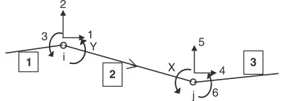
Figure 1.1shows a frame with 7 degrees of freedom. Note that the pinned joint at C allows the two members BC and CD to rotate indepen-dently, thus giving rise to two freedoms in rotation at the joint.
In structural analysis, the degree of statical indeterminacy is important, as its value may determine whether the structure
1
7 3
2
4 6
5
B C
D A
FIGURE 1.1. Degrees of freedom of a frame.
is globally unstable or stable. If the structure is stable, the degree of statical indeterminacy is, in general, proportional to the level of com-plexity for solving the structural problem.
The method described here for determining the degree of statical indeterminacy of a structure is based on that by Rangasami and Mallick.6
Only plane frames will be dealt with here, although the method can be extended to three-dimensional frames.
1.2.1 Degree of Statical Indeterminacy of Frames
For a free member in a plane frame, the number of possible displace-ments is three: horizontal, vertical, and rotational. If there aren mem-bers in the structure, the total number of possible displacements, denoted bym, before any displacement restraints are considered, is
m¼3n (1.1)
For two members connected at a joint, some or all of the displa-cements at the joint are common to the two members and these com-mon displacements are considered restraints. In this method for determining the degree of statical indeterminacy, every joint is con-sidered as imposingrnumber of restraints if the number of common displacements between the members is r. The ground or foundation is considered as a noncounting member and has no freedom.Figure 1.2 indicates the value ofr for each type of joints or supports in a plane frame.
For pinned joints with multiple members, the number of pinned joints, p, is counted according toFigure 1.3. For example, for a four-member pinned connection shown in Figure 1.3, a first joint is counted by considering the connection of two members, a second joint by the third member, and so on. The total number of pinned joints for a four-member connection is therefore equal to three. In gen-eral, the number of pinned joints connectingnmembers isp¼n –1. The same method applies to fixed joints.
r = 1 (a) Roller
r = 2 (b) Pin
r = 3 (c) Fixed
r = 2 (d) Pin
r = 3 (e) Rigid (≡ fixed)
For a connection at a roller support, as in the example shown in Figure 1.4, it can be calculated thatp¼2.5 pinned joints and that the total number of restraints isr¼5.
The degree of statical indeterminacy,fr, of a structure is
deter-mined by
fr¼m
X
r (1.2)
a. Iffr¼0, the frame is stable and statically determinate.
b. Iffr<0, the frame is stable and statically indeterminate to the
degreefr.
c. Iffr>0, the frame is unstable.
Note that this method does not examine external instability or partial collapse of the structure.
Example 1.1 Determine the degree of statical indeterminacy for the pin-jointed truss shown inFigure 1.5.
No. of pins, p = 1 No. of pins, p = 2 No. of pins, p = 3
FIGURE 1.3. Method for joint counting.
No. of pins, p = 2.5
FIGURE 1.4. Joint counting of a pin with roller support.
(a) (b)
FIGURE 1.5. Determination of degree of statical indeterminacy in Example 1.1.
Soluti on. For th e truss in Figure 1.5a , number of membe rs n ¼ 3; num-ber of pinned joints p ¼ 4.5.
Hence, fr ¼ 3 3 2 4:5 ¼ 0 and the truss is a determ inate
struct ure. For the truss in Figure 1.5b , num ber of membe rs n ¼ 2; numb er of pinn ed joints p ¼ 3.
Hence, fr ¼ 3 2 2 3 ¼ 0 a nd the truss is a determ inate
struct ure.
Examp le 1.2 Dete rmine the de gree of stati cal indeter minacy for the frame with mixed pin and rigid joint s sho wn in Figu re 1.6 .
Soluti on. For this frame, a membe r is c ounted as one betwe en two adjace nt joint s. Numbe r of membe rs ¼ 6; number of rigi d (or fixed) joints ¼ 5. Note that the joint betwe en DE and EF is a rigi d one, where as the joint betwe en BE an d DEF is a pinn ed one . Number of pinned joints ¼ 3.
Hence, fr ¼ 3 6 3 5 2 3 ¼ 3 and the fram e is an
inde-term inate struct ure to the de gree 3.
1.3 Statically Indeterminate Structures—Direct
Stiffness Method
The spring system shown in Figure 1.7 demon strates the use of the stiffnes s method in its simplest form . The single degree of freedom struct ure consis ts of an object suppo rted by a linear spring obey ing Hooke’s law. For structural analysis, the weight,F, of the object and the spring constant (or stiffness),K, are usually known. The purpose
A B C
E D
F
of the structural analysis is to find the vertical displacement,D, and the internal force in the spring,P.
From Hooke’s law,
F¼KD (1.3)
Equation (1.3)is in fact the equilibrium equation of the system. Hence, the displacement,D, of the object can be obtained by
D¼F=K (1.4)
The displacement,d, of the spring is obviously equal toD. That is,
d¼D (1.5)
The internal force in the spring,P, can be found by
P¼Kd (1.6)
In this simple example, the procedure for using the stiffness method is demonstrated throughEquations (1.3) to (1.6). For a struc-ture composed of a number of structural members with ndegrees of freedom, the equilibrium of the structure can be described by a num-ber of equations analogous toEquation (1.3). These equations can be expressed in matrix form as
F
f gn1¼½ Knnf gD n1 (1.7) wheref gF n1is the load vector of sizeðn1Þcontaining the external loads, ½ Knn is the structure stiffness matrix of size ðnnÞ
corresponding to the spring constant K in a single degree system shown in Figure 1.7, and f gD n1 is the displacement vector of size
n1
ð Þ containing the unknown displacements at designated loca-tions, usually at the joints of the structure.
K
F
D
FIGURE 1.7. Load supported by linear spring.
The unknown displacement vector can be found by solving Equation (1.7)as
D
f g ¼½ K 1f gF (1.8)
Details of the formation off gF ,½ K, andf gD are given in the following sections.
1.3.1 Local and Global Coordinate Systems
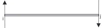
A framed structure consists of discrete members connected at joints, which may be pinned or rigid. In a local coordinate system for a mem-ber connecting two joints i and j, the member forces and the corresponding displacements are shown inFigure 1.8, where the axial forces are acting along the longitudinal axis of the member and the shear forces are acting perpendicular to its longitudinal axis.
In Figure 1.8, Mi,j, yi,j ¼ bending moments and corresponding
rotations at ends i, j, respectively; Ni,j, ui,j are axial forces and
corresponding axial deformations at ends i, j, respectively; and Qi,j, vi,j are shear forces and corresponding transverse displacements at
endsi, j, respectively. The directions of the actions and movements shown inFigure 1.8are positive when using the stiffness method.
As mentioned inSection 1.2, the freedom codes of a structure are assigned in its global coordinate system. An example of a member forming part of the structure with a set of freedom codes (1, 2, 3, 4, 5, 6) at its ends is shown inFigure 1.9. At either end of the member, the direction in which the member is restrained from movement is assigned a freedom code “zero,” otherwise a nonzero freedom code is assigned. The relationship for forces and displacements between local and global coordinate systems will be established in later sections.
i
j
Mj, qj Nj, uj Qj, vj
Mi, qi N
i, ui
Qi, vi
1.4 Member Stiffness Matrix
The structure stiffness matrix ½ K is assembled on the basis of the equilibrium and compatibility conditions between the members. For a general frame, the equilibrium matrix equation of a member is
P
f g ¼½Kef gd (1.9)
where f gP is the member force vector, ½Ke is the member stiffness
matrix, andf gd is the member displacement vector, all in the mem-ber’s local coordinate system. The elements of the matrices in Equa-tion (1.9)are given as
P
1.4.1 Derivation of Elements of Member Stiffness Matrix
A member under axial forces Ni and Nj acting at its ends produces
axial displacements ui and uj as shown in Figure 1.10. From the
stress-strain relation, it can be shown that
Ni ¼EA
where E is Young’s modulus, A is cross-sectional area, and L is length of the member. Hence,K11¼ K14¼ K41 ¼K44¼
EA L .
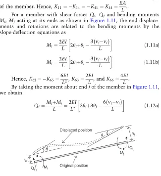
For a member with shear forces Qi, Qj and bending moments Mi, Mj acting at its ends as shown in Figure 1.11, the end
displace-ments and rotations are related to the bending modisplace-ments by the slope-deflection equations as
Mi¼
2EI
L 2yiþyj
3 vj vi
L
(1.11a)
Mj¼
2EI
L 2yjþyi
3 vj vi
L
(1.11b)
Hence,K62¼ K65¼ 6EI
L2,K63¼ 2EI
L , andK66¼ 4EI
L .
By taking the moment about endjof the member inFigure 1.11, we obtain
Qi ¼
MiþMj
L ¼ 2EI
L2 3yiþ3yj
6 vj vi
L
(1.12a) i
j
Ni
ui
uj
Nj
Original position
Displaced position
FIGURE 1.10. Member under axial forces.
qi
vi
vj
Qj
Original position Displaced position
qj
Qi Mi
Mj
i
j
Also, by taking the moment about endiof the member, we obtain Qj ¼
MiþMj
L
¼ Qi (1.12b)
Hence,
K22¼K55¼ K25¼ K52¼ 12EI
L3 and K23¼K26¼ K53¼ K66¼ 6EI
L2. In summary, the resulting member stiffness matrix is symmetric about the diagonal:
Ke
½ ¼
EA
L 0 0
EA
L 0 0
0 12EI
L3
6EI L2 0
12EI L3
6EI L2
0 6EI
L2
4EI
L 0
6EI L2
2EI L EA
L 0 0
EA
L 0 0
0 12EI
L3
6EI L2 0
12EI L3
6EI L2
0 6EI
L2
2EI
L 0
6EI L2
4EI L 2
6 6 6 6 6 6 6 6 6 6 6 6 6 6 6 6 6 6 6 6 6 6 4
3 7 7 7 7 7 7 7 7 7 7 7 7 7 7 7 7 7 7 7 7 7 7 5
(1.13)
1.5 Coordinates Transformation
In order to establish the equilibrium conditions between the member forces in the local coordinate system and the externally applied loads in the global coordinate system, the member forces are transformed into the global coordinate system by force resolution. Figure 1.12 shows a member inclined at an angleato the horizontal.
1.5.1 Load Transformation
The forces in the global coordinate system shown with superscript “g” inFigure 1.12are related to those in the local coordinate system by
Hgi ¼Nicosa Qisina (1.14a)
Vgi ¼NisinaþQicosa (1.14b)
Mig¼Mi (1.14c)
Similarly,
Hgj ¼Njcosa Qj sina (1.14d)
Vgj ¼Nj sinaþQjcosa (1.14e)
Mgj ¼Mj (1.14f)
In matrix form,Equations (1.14a) to (1.14f) can be expressed as Fg
e
¼½ Tf gP (1.15)
wheref gFge is the member force vector in the global coordinate system
and½ T is the transformation matrix, both given as
Fg e
¼
Hig Vig Mgi Hjg Vjg Mgj 8 > > > > > > > > > < > > > > > > > > > :
9 > > > > > > > > > = > > > > > > > > > ;
and½ ¼T
cosa sina 0 0 0 0
sina cosa 0 0 0 0
0 0 1 0 0 0
0 0 0 cosa sina 0
0 0 0 sina cosa 0
0 0 0 0 0 1
2 6 6 6 6 6 6 6 6 4
3 7 7 7 7 7 7 7 7 5
:
1.5.2 Displacement Transformation
The displacements in the global coordinate system can be related to those in the local coordinate system by following the procedure simi-lar to the force transformation. The displacements in both coordinate systems are shown inFigure 1.13.
FromFigure 1.13,
ui ¼ugi cosaþv g
i sina (1.16a)
i
Mi Ni
Qi
Mj Nj
Qj
Mgi Vgi
Hgi
j
Mgj
Vgj
Hgj
α
vi ¼ ugi sinaþvgi cosa (1.16b)
yi ¼yg
i (1.16c)
uj¼ugj cosaþv g
j sina (1.16d)
vj ¼ ugj sinaþv g
j cosa (1.16e)
yj¼yg
j (1.16f)
In matrix form,Equations (1.16a) to (1.16f) can be expressed as d
f g ¼½ Tt Dge
(1.17) where fDgeg is the member displacement vector in the global
coordi-nate system corresponding to the directions in which the freedom codes are specified and is given as
Dge
¼
ugi vig yg
i
ugj vjg yg
j
8 > > > > > > > > > < > > > > > > > > > :
9 > > > > > > > > > = > > > > > > > > > ; and½ Ttis the transpose of½ T.
1.6 Member Stiffness Matrix in Global Coordinate System
FromEquation (1.15),Fg e
¼½ Tf gP
¼½ T½Kef gd from Equation ð 1: 9Þ
uj vj
vgi
ugi
α θi
θj
ui vi
vgj
ugj
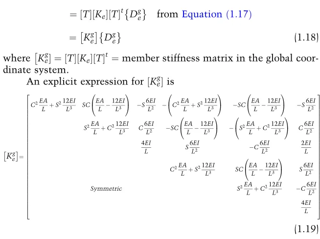
¼ T½ ½Ke½ Tt D ge
dinate system.
An explicit expression for½Kegis
Symmetric S2EA
LþC
1.7 Assembly of Structure Stiffness Matrix
Consider part of a structure with four externally applied forces, F1, F2, F4, and F5, and two applied moments, M3 and M6, acting at the two jointspandqconnecting three members A, B, and C as shown in Figure 1.14. The freedom codes at jointpare {1, 2, 3} and at jointqare {4, 5, 6}. The structure stiffness matrix [K] is assembled on the basis of two conditions: compatibility and equilibrium conditions at the joints.
1.7.1 Compatibility Condition
At jointp, the global displacements areD1 (horizontal),D2 (vertical), andD3 (rotational). Similarly, at jointq, the global displacements are D4 (horizontal), D5 (vertical), and D6 (rotational). The compatibility condition is that the displacements (D1,D2, andD3) at endpof
The member stiffness matrix in the global coordinate system given inEquation (1.19)can be written as
Kge
¼
k11 k12 k13 k14 k15 k16 k21 k22 k23 k24 k25 k26 k31 k32 k33 k34 k35 k36 k41 k42 k43 k44 k45 k46 k51 k52 k53 k54 k55 k56 k61 k62 k63 k64 k65 k66 2
6 6 6 6 6 6 4
3 7 7 7 7 7 7 5
(1.20)
wherek11¼C2 EA
L þS 212EI
L3 , etc.
For member A, fromEquation (1.18), Hgj
A¼:::::þ:::::þ:::::þðk44ÞAD1þðk45ÞAD2þðk46ÞAD3 (1.21a)
Vjg
A¼:::::þ:::::þ:::::þðk54ÞAD1þðk55ÞAD2þðk56ÞAD3 (1.21b)
Mgj
A¼:::::þ:::::þ:::::þðk64ÞAD1þðk65ÞAD2þðk66ÞAD3 (1.21c)
Similarly, for member B, Hgi
B¼ðk11ÞBD1þðk12ÞBD2þðk13ÞBD3þðk14ÞBD4þðk15ÞBD5þðk16ÞBD6
(1.21d) Vig
B¼ðk21ÞBD1þðk22ÞBD2þðk23ÞBD3þðk24ÞBD4þðk25ÞBD5þðk26ÞBD6
(1.21e)
Mgi
B¼ðk31ÞBD1þðk32ÞBD2þðk33ÞBD3þðk34ÞBD4þðk35ÞBD5þðk36ÞBD6
(1.21f)
2
1 3
4 5
6
p
q
F1
F2
F4
F5
A
B C
M3
M6
FIGURE 1.14. Assembly of structure stiffness matrix [K].
Hjg
B¼ðk41ÞBD1þðk42ÞBD2þðk43ÞBD3þðk44ÞBD4þðk45ÞBD5þðk46ÞBD6
(1.21g) Vjg
B¼ðk51ÞBD1þðk52ÞBD2þðk53ÞBD3þðk54ÞBD4þðk55ÞBD5þðk56ÞBD6
(1.21h) Mjg
B¼ðk61ÞBD1þðk62ÞBD2þðk63ÞBD3þðk64ÞBD4þðk65ÞBD5þðk66ÞBD6
(1.21i) Similarly, for member C,
Hgi
C¼ðk11ÞCD1þðk12ÞCD2þðk13ÞCD3þ:::::þ:::::þ::::: (1.21j) Vgi
C¼ðk21ÞCD1þðk22ÞCD2þðk23ÞCD3þ:::::þ:::::þ::::: (1.21k) Mgi
C¼ðk31ÞCD1þðk32ÞCD2þðk33ÞCD3þ:::::þ:::::þ::::: (1.21l)
1.7.2 Equilibrium Condition
Any of the externally applied forces or moments applied in a certain direction at a joint of a structure is equal to the sum of the member forces acting in the same direction for members connected at that joint in the global coordinate system. Therefore, at jointp,
F1¼Hgj
Aþ H
g i
B (1.22a)
F2¼Vjg
Aþ V
g i
B (1.22b)
M3¼Mgj
Aþ M
g i
B (1.22c)
Also, at joint q,
F4¼Hgj
Bþ H
g i
C (1.22d)
F5¼Vjg
Bþ V
g i
C (1.22e)
M6¼Mgj
Bþ M
g i
C (1.22f)
where the “l” stands for matrix coefficients contributed from the
other parts of the structure. In simple form, Equation (1.23) can be written as
F
f g ¼½ Kf gD
which is identical to Equation (1.7). Equation (1.23) shows how the structure equilibrium equation is set up in terms of the load vector
F
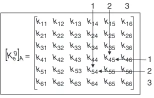
f g, structure stiffness matrix½ K, and the displacement vectorf gD . Close examination of Equation (1.23) reveals that the stiffness coefficients of the three members A, B, and C are assembled into½ K in a way according to the freedom codes assigned to the members. Take member A as an example. By writing the freedom codes in the order of endsiandjaround the member stiffness matrix in the global coordinate system shown inFigure 1.15, the coefficient, for example, k54, is assembled into the position [2, 1] of½ K. Similarly, the coeffi-cientk45 is assembled into the position [1, 2] of½ K. The coefficients in all member stiffness matrices in the global coordinate system can be assembled into½ K in this way. Since the resulting matrix is sym-metric, only half of the coefficients need to be assembled.
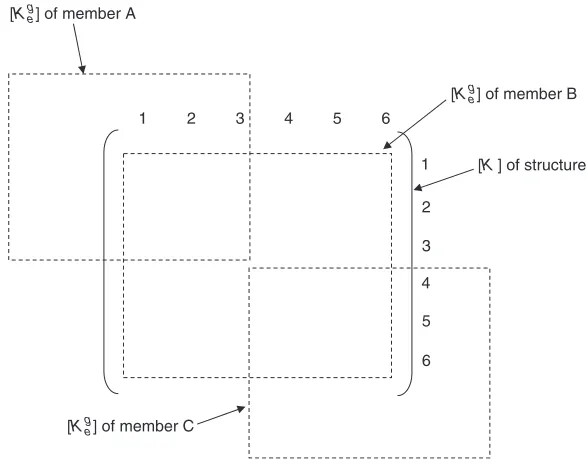
A schematic diagram showing the assembly procedure for the stiffness coefficients of the three members A, B, and C into ½ K is shown in Figure 1.16. Note that since ½Keg is symmetric, ½ K is also
symmetric. Any coefficients in a row or column corresponding to zero freedom code will be ignored.
1.8 Load Vector
The load vectorf gF of a structure is formed by assembling the individ-ual forces into the load vector in positions corresponding to the direc-tions of the freedom codes. For the example in Figure 1.14, the load factor is given as that shown inFigure 1.17.
[
Keg]
A =k66 k65 k64 k63 k62 k61
k56 k55 k54 k k52 k51
k46 k45 k44 k43 k42 k41
k36 k35 k34 k33 k32 k31
k26 k25 k24 k23 k22 k21
k16 k15 k14 k13 k12 k11
1 2 3
1 2 3
53
1.9 Methods of Solution
The displacements of the structure can be found by solvingEquation (1.23). Because of the huge size of the matrix equation usually encoun-tered in practice, Equation (1.23) is solved routinely by numerical methods such as the Gaussian elimination method and the iterative Gauss–Seidel method. It should be noted that in using these
{
F}
=• •
6 5 4 3 2 1
F F F F F F
Freedom codes
1 2 3 4 5 6
FIGURE 1.17. Assembly of load vector.
1 2 3 4 5 6
1
2
3
4
5
6 [Kge] of member A
[Kge] of member C
[Kge] of member B
[K] of structure
FIGURE 1.16. Assembly of structure stiffness matrix.
numerical methods, the procedure is analogous to inverting the struc-ture stiffness matrix, which is subsequently multiplied by the load vector as inEquation (1.8):
D
f g ¼½ K 1f gF (1.8)
The numerical procedure fails only if an inverted½ K cannot be found. This situation occurs when the determinant of ½ K is zero, implying an unstable structure. Unstable structures with a degree of statically indeterminacy, fr, greater than zero (see Section 1.2) will
have a zero determinant of½ K. In numerical manipulation by compu-ters, an exact zero is sometimes difficult to obtain. In such cases, a good indication of an unstable structure is to examine the displace-ment vector f gD , which would include some exceptionally large values.
1.10 Calculation of Member Forces
Member forces are calculated according toEquation (1.9). Hence, P
f g ¼½Kef gd ¼½Ke½ TtfDgeg
(1.24)
where fDgeg is extracted from f gD for each member according to its
freedom codes and
Ke
P
In summary, the procedure for using the stiffness method to calculate the displacements of the structure and the member forces is as follows.
1. Assign freedom codes to each joint indicating the displace-ment freedom at the ends of the members connected at that joint. Assign a freedom code of “zero” to any restrained displacement.
2. Assign an arrow to each member so that ends i and j are defined. Also, the angle of orientation a for the member is
defined inFigure 1.18as:
3. Assemble the structure stiffness matrix½ K from each of the member stiffness matrices.
4. Form the load vectorf gF of the structure. i
j
α
FIGURE 1.18. Definition of angle of orientation for member.
5. Calculate the displacement vector f gD by solving for D
f g ¼½ K 1f gF .
6. Extract the local displacement vectorfDgeg fromf gD and
cal-culate the member force vectorf gP usingf g ¼P ½Ke½ TtfDgeg.
1.10.1 Sign Convention for Member Force Diagrams
Positive member forces and displacements obtained from the stiffness method of analysis are shown inFigure 1.19. To plot the forces in con-ventional axial force, shear force, and bending moment diagrams, it is necessary to translate them into a system commonly adopted for plotting.
The sign convention for such a system is given as follows.
Axial Force
For a member under compression, the axial force at endi is positive (from analysis) and at end j is negative (from analysis), as shown in Figure 1.20.
Shear Force
A shear force plotted positive in diagram is acting upward (positive from analysis) at end i and downward (negative from analysis) at endj as shown inFigure 1.21. Positive shear force is usually plotted in the space above the member.
FIGURE 1.19. Direction of positive forces and displacements using stiffness method.
Compressive
i j
Bendin g Moment
A membe r under saggin g momen t is pos itive in diagra m (clockwi se and ne gative from an alysis) at end i and pos itive (anti clockwise and pos-itive from analysis) at e nd j as shown in Figure 1.22 . Pos itive bending moment is usually plotte d in the space beneath the membe r. In doing so, a be nding moment is plo tted on the tensi on face of the membe r.
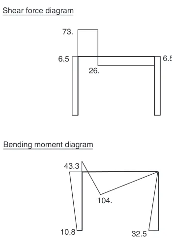
Example 1.3 Determi ne the membe r forces and plot the shear force and bend ing moment diagra ms for the struct ure shown in Figure 1.23 a. The struct ure with a pin at D is subjec t to a verti cal force of 100 kN being ap plied at C. For all membe rs, E ¼ 2 108 kN/m 2 , A ¼ 0.2 m 2 , and I ¼ 0.001 m 4.
Soluti on. The freedom codes for the whole struct ure are shown in Figure 1.23b . There are four membe rs separat ed by joint s B, C, and D wit h the membe r num bers shown. The arrows are assigned to
i j
FIGURE 1.21. Positive shear forces.
i j
FIGURE 1.22. Sagging moment of a member.
7 4
6 5
B D
8
1 3
2
9
10
A C
E 0
0 0
0 0
0
1
2 3
4
B
C
A
D
E 100 kN
5m
2m 4m
(a) Frame with applied load (b) Freedom codes
FIGURE 1.23. Example 1.3.
indicate endi(tail of arrow) and endj(head of arrow). Thus, the orien-tations of the members are
Member 1:a¼90
Member 2:a¼0
Member 3:a¼0
Member 4:a¼270 or –90
The ½Keg for the members with the assigned freedom codes for
the coefficients is
0 0 0 1 2 3
By assembling from½Keg of all members, the structure stiffness
K
½ ¼
2:0019107 0 4:8104 2107 0 0 0 0 0 0
8:3106 3105 0 3105 3105 0 0 0 0
5:6105 0 3105 2105 0 0 0 0
3107 0 0 1107 0 0 0
3:375105 2:25105 0 3:75104 7:5104 0
6105 0 7:5104 1105 0
1:0019107 0 0 4:8104
Symmetric 8:0375106 7:5104 0
2105 0
1:6105
2 6 6 6 6 6 6 6 6 6 6 6 6 6 6 4
3 7 7 7 7 7 7 7 7 7 7 7 7 7 7 5
Structural
Analysis—Stiffness
Method
The shear force and bending moment diagrams are shown in Figure 1.24.
1.11 Treatment of Internal Loads
So far, the discussion has concerned externally applied loads acting only at joints of the structure. However, in many instances, externally applied loads are also applied at locations other than the joints, such as on part or whole of a member. Loads being applied in this manner are termed internal loads. Internal loads may include distributed loads, point loads, and loads due to temperature effects. In such cases, the loads are calculated by treating the member as fixed-end, and fixed-end forces, including axial forces, shear forces, and bending moments, are calculated at its ends. The fictitiously fixed ends of the member are then removed and the effects of the fixed-end forces, now being treated as applied loads at the joints, are assessed using the stiffness method of analysis.
InFigure 1.25, fixed-end forces due to the point load and the uni-formly distributed load are collected in a fixed-end force vector fPFg
for the member as
6.5 6.5
73.
26.
10.8 43.3
104.
32.5 Shear force diagram
Bending moment diagram
FIGURE 1.24. Shear force and bending moment diagrams.
PF
f g ¼
0 QFi
MFi
0 QFj
MFj
8 > > > > > > < > > > > > > :
9 > > > > > > = > > > > > > ;
(1.25)
The signs of the forces infPFg should follow those shown in Figure
1.19. In equilibrium, fixed-end forces generate a set of equivalent forces, equal in magnitude but opposite in sense and shown as QEi,
MEi, QEj, MEj, being applied at the joints pertaining to both ends i
andjof the member. The equivalent force vector is expressed as
PE
f g ¼
0 QFi
MFi
0 QFj
MFj
8 > > > > > > < > > > > > > :
9 > > > > > > = > > > > > > ;
(1.26)
If necessary,fPEg is transformed into the global coordinate
sys-tem in a similar way given inEquation (1.15)to form PgE
¼½ TfPEg (1.27)
which is added to the load vector f gF of the structure in accordance with the freedom codes at the joints. Final member forces are calcu-lated as the sum of the forces obtained from the global structural anal-ysis and fixed-end forcesfPFg. That is,
P
f g ¼½Kef g þd fPFg (1.28)
Fixed-end forces for two common loading cases are shown in Table 1.1.
Example 1.4Determine the forces in the members and plot the bend-ing moment and shear force diagrams for the frame shown in Figure 1.26a. The structure is fixed at A and pinned on a roller support
i j
100 kN
20 kN/m QFi
MFi
QFj
MEj
MFj
QEj
MEi QEi
TABLE 1.1 Fixed-end forces
i j
w (load/length)
b
a c
L
Shear force at endi,QFi QFi¼
wb b
2þc
L þ
MFiþMFj L
Shear force at endj,QFj QFj¼wb QFi
Bending moment at endi,MFi MFi¼
w
12L2 ðL aÞ
3ðLþ3aÞ c3ð4L 3cÞ
h i
Bending moment at endj,MFj MFj¼
w
12L2 ðL cÞ
3ðLþ3cÞ a3ð4L 3aÞ
h i
P
i a b j
L
Shear force at endi,QFi QFi¼P
b L
2 1þ2a
L
Shear force at endj,QFj QFj¼P QFi
Bending moment at endi,MFi M
Fj¼ Pab2
L2
Bending moment at endj,MFj MFj¼
Pa2b
L2
Structural
Analysis—Stiffness
Method
at C. For bot h membe rs AB an d BC, E ¼ 2 108 kN/m 2 , A ¼ 0.2 m 2 , I ¼ 0.001 m 4 .
Soluti on. The struct ure has 5 degrees of freedom with a de gree of stat-ical indeter minac y of 2. Freed om co des corresp onding to the 5 degrees of freedom are shown in Figure 1.26 b. The fixed-end force vector for membe r 1 is The equival ent force vector is
PE whic h is ad ded to the external ly app lied force to form
F
dinate system are B
(a) Frame with applied load (b) Freedom
0 0 0 1 2 3
Hence, the structure stiffness matrix is assembled as
K
By solving the structure equilibrium equation, the displacement vec-tor is determined as
D
The shear force and bending moment diagrams of the structure are shown inFigure 1.27.
1.12 Treatment of Pins
Examp le 1.3 demonst rates the ana lysis of a fram e wit h a pin at joint D. The way to treat the pin using the stiffnes s method for struct ural anal-ysis is to allow the membe rs attache d to the pinned joint to rotate indepen dently, thus leadi ng to the creation of differen t freedom code s for rotati ons of indivi dual membe rs. When carryin g out e lastoplast ic analysi s (Chapter 4) for struct ures using the stiffnes s method, th e plast ic hinges, behaving in a way simila r to a pin, are form ed in stages as the loads increa se. In assign ing different freedom code s to repres ent the creation of plastic hinges in an elasto plastic analysis, the numb er of degrees of freedom increa ses by one every time a plast ic hinge is form ed. For a struct ure with a high degree of statical indeter minac y, the increa se in th e number of freedom c odes from the be ginning of the elast oplast ic analysis to its colla pse due to instab ility induced by th e formation of plast ic hinges may be large . Elasto plastic analysi s using this method for simu lating pin be havior, hereaf ter call ed the extra freedom method, therefo re requ ires increa sing both the numb er of equilibri um e quations to be solved and the size of the struct ure stiffnes s matrix ½ K, thus increa sing the storag e requir ements for the compu ter and decreas ing the efficie ncy of the soluti on procedu re. In order to maint ain the size of ½ K a nd maxim ize comp utation al effi-ciency in an elastop lastic an alysis, the beh avior of a pin at the end s of the membe r can be sim ulated implici tly by mod ifying the membe r stiffnes s matr ix ½Ke. This latter method for pin beh avior sim ulated
implici tly in the membe r stiffnes s matrix is call ed the condensati on method, which is described ne xt.
1.12.1 Condensation Method
The rotatio nal freedom for an y membe r can be express ed exp licitly outside the domain of the stiffnes s matrix. In doin g so, the rotati onal
C B
A 90.8
42.8
26.3
26.3 C
B A
155.5
111.7 111.7
(a) Shear force diagram (b) Bending moment
freedom is regarded as a variable dependent on other displacement quantities and can be eliminated from the member stiffness matrix. The process of elimination is calledcondensationand hence the name of this method.
In using the condensation method, while the stiffness matrix of the member needs to be modified according to its end connection con-dition, the internal loads associated with that member also need to be modified. There are three cases that need to be considered for a mem-ber. They are (i) pin at endj, (ii) pin at endi, and (iii) pins at both ends.
Case i: Pin at endj
Consider part of a structure shown inFigure 1.28. The freedom codes for member 2 with a pin at end jare 1f ;2;3;4;5;Xg where the rota-tional freedomXis treated as a dependent variable outside the struc-ture equilibrium equation, leaving the member with only 5 freedom codes pertaining to the structure stiffness matrix ½ K. Note that the rotational freedom code ‘6’ belongs to member 3.
FromEquation (1.28)for member 2 with internal loads,
Ni
where the rotation at endjisyjXcorresponding to a rotational freedom code ‘X’. Expanding the last equation in Equation (1.29) and given MjX¼0 for a pin,yjX can be derived as
By substitutingEquation (1.30)into the other equations of Equa-tion (1.29), a modified 5 5 member stiffness matrix, Kej, and a
modified fixed-end force vector,fPFjg, for a member with pin at endj are obtained:
Ni
The member stiffness matrix in the global coordinate system can be derived as before using a modified transformation matrix, Tj,
which is given as
Tj
Accordingly, for a member with a pin at endj, the member stiff-ness matrix in the global coordinate system is
Kejg
Symmetric S2EA
L þC The modified fixed-end force vector in the global coordinate sys-tem,fPgEjg, can be derived in a way similar toEquation (1.27).
There are two ways to calculate the member forces. The first way is to useEquation (1.24), for which the end rotation at end j of the member in fDgeg is replaced by yjX calculated from Equation
(1.30). The second way is to use a form similar toEquation (1.24): P where, throughEquations (1.32) and (1.34),
Kej
The 51 member displacement vectorfDgeginEquation (1.36a)
is extracted fromf gD according to the 5 freedom codes 1f ;2;3;4;5g shown inFigure 1.28for the member.
Case ii: Pin at endi
This case is shown inFigure 1.29where member 2 has a pin at endi with an independent rotational freedom code Y. The freedom codes for member 2 with a pin at endiare 1f ;2;Y;4;5;6g. Note that the free-dom code 3 belongs to member 1.
By writing
The corresponding matrices for this case can be derived in a way similar to Caseimentioned earlier. The results are
Ni
Equation (1.40) repres ents the supp ort reactio ns equ al to those of a propped cantilever beam. Explicit expressions for the coefficients in
Accordingly, for the member with pin at endi, the member stiff-ness matrix in the global coordinate system is
Kgei
Symmetric 3EI
L
The 5 1 member displacement vector fDgeg is extracted from
D
f gaccording to the 5 freedom codes 1f ;2;4;5;6gfor the member.
Case iii: Pins at both endsiandj
In this case, substitute MiY ¼MjX¼0 into Equation (1.29), we
Equation (1.47)represents the support reactions equal to those of a simply supported beam. Explicit expressions for the coefficients in
PFij
are given in Table 1.2 in Section 1.12 .1.4 .
It is noted that Keij is in fact the stiffness matrix of a truss
member. The transformation matrix for the member in this case is
Tij
The corresponding stiffness matrix in the global coordinate sys-tem for a member with pins at both ends is
and
Kgeij
h i
Tij
t
¼EA
L
C S C S
0 0 0 0
C S C S
0 0 0 0
2 6 6 4
3 7 7 5
(1.50)
Modified Fixed-End Force Vector
The explicit expressions for the coefficients of the modified fixed-end force vectors given inEquations (1.33), (1.40), and (1.47)are summar-ized inTable 1.2.
TABLE 1.2
Modified fixed-end forces for members with pins
j i
w (load/length)
b
a c
L
Q0Fi ¼wb
b
2þc
L þ
M0Fi L Q0
Fj ¼wb Q
0
Fi M0Fi ¼ w
8L2 ðbþ2cÞb 2L
2 c2 ðbþcÞ2
h i
P
i j
b a
L
Q00Fi ¼P Q00Fj Q00Fj ¼Pa
2
2L3ðbþ2LÞ
M00Fi ¼Pb L
2 b2
2L2
Moment under load
¼Pb
2 2
3b L þ
b3
L3
i
w (load/length)
b
a c
L
Q000Fi ¼wb L
b
2þc
Q000
Fj ¼
wb L
b
2þa
Mmax ¼w
x2 a2
2
atx¼aþQ
000
Fi w P
i j
b a
L
Q000Fi ¼Pb L
Q000Fj ¼Pa L Moment
under load
¼Pab
Procedure for Using Condensation Method
1. For any joints with pins, determine whether the connecting members have (a) no pin, (b) pin at end i, (c) pin at endj, or (d) pins at both ends.
2. Use the appropriate stiffness matrix for the cases just given for all members.
3. Assign freedom codes to each joint.
4. Assemble the structure stiffness matrix½ K.
5. After solving the structure equilibrium equation, calculate the angle of rotation yjX or yiY for each pin using Equations (1.30), (1.37), or (1.44). Calculate the member forces accordingly.
1.12.2 Methods to Model Pin
There are a number of ways to model a joint with a pin using the for-mulations given in the previous section. Consider a pinned joint con-necting two members 1 and 2. There are four ways of formulation for use in the stiffness method of analysis as shown in Figure 1.31. Figure 1.31ais based on the extra freedom method where both mem-bers 1 and 2 have independent rotations D3 and D4 using the full
66 member stiffness matrix.Figure 1.31bis based on the condensa-tion method for member 1 using the formulacondensa-tion for pin at end j as given in Section 1.12.1.1, whereas member 2 retains use of the full 66 member stiffness matrix.Figure 1.31cis also based on the con-densation method for member 2 using the formulation for pin at endi
X 3
1 2
1
2
3 Y
1 2
1
2
X Y
1 2
1
2
3 4
1 2
1
2
(a) (b)
(c) (d)
FIGURE 1.31. Modeling pin at a joint.
as given in Section 1.12.1 .2, where as membe r 1 retai ns use of the full 6 6 membe r stiffnes s matr ix. Figure 1.31d is based on the con densa-tion method using the formulati on for pin at end j for membe r 1 and pin at end i for membe r 2.
Examp le 1.5 Dete rmin e the displ acement s and forces in the beam ABC wit h a pin at B shown in Figure 1.32 . Ignore the effe ct of axial force. E ¼ 2000 kN/m 2 , I ¼ 0.015 m 4 .
Soluti on
(i) Extra Freedom Meth od
When the axial force effect is ignored , a zero freedom cod e is assig ned to the axial deform ation of the membe rs. Thus, the struct ure has a total of 3 degrees of freedom shown in Figure 1.32b .
For all matr ices, only the coeffici ents co rrespondi ng to nonze ro freedom codes will be sho wn.
For membe r 1,
0 0 0 0 1 2
K eg ½ 1 ¼
:: :: :: :: :: :: :: :: :: :: :: :: :: :: :: :: :: ::
Symmet ric 5 :625 11 :25 30 2
6 6 6 6 6 6 4
3 7 7 7 7 7 7 5 0 0 0 0 1 2 For membe r 2,
0 1 3 0 0 0
Keg
½ 2¼
:: :: :: :: :: ::
45 45 :: :: ::
60 :: :: :: :: :: ::
Symmetric :: :: ::
2 6 6 6 6 6 6 4
3 7 7 7 7 7 7 5 0 1 3 0 0 0
(a) Beam with pin at B (b) Freedom codes−Extra Freedom Method
B C
A
5 kN
2m 4m
0 00
C 0
0 0
B A
1 2
0
2 1
3
Hence,
Figure 1.33shows the deflection and rotations of the members.
The member forces for member 1 are
P The member forces for member 2 are
P The member forces for the structure are shown inFigure 1.34.
C
B
A 0.395 m
0.296 0.148
FIGURE 1.33. Deflection and rotations.
2.223 kNm
0.556 kN
4.444 kN 8.891 kNm
4.444 kN 0.556 kN
FIGURE 1.34. Member forces.
(ii) Method of Condensation
In using this method, the stiffness matrix of member 1 is condensed so that rotation at end j, denoted as X in Figure 1.35, becomes a dependent variable. The freedom codes of the structure are also shown inFigure 1.35.
The stiffness matrix of member 1 is given byEquation (1.32)as
0 0 0 0 1
Kej
1¼ K
g ej
h i
1¼
:: :: :: :: ::
:: :: :: ::
:: :: ::
Symmetric ::
1:4063 2
6 6 6 6 4
3 7 7 7 7 5 0 0 0 0 1 For member 2,
0 1 2 0 0 0
Keg
½ 2¼
:: :: :: :: :: ::
45 45 :: :: ::
60 :: :: :: :: :: ::
Symmetric :: :: ::
2 6 6 6 6 6 6 4
3 7 7 7 7 7 7 5 0 1 2 0 0 0
Hence, the structure stiffness matrix, of size 22, can be assem-bled as
K
½ ¼ 4645:406 4560
The load vector is
F
f g ¼ 05
By solvingf g ¼F ½ Kf gD forf gD , we obtain D
f g ¼ DD1
2
¼ 00:395
:296
0 0
0
C 0
0 0
B A
1 2
0
X 1
2
The rotationyjXfor member 1 can be obtained fromEquation (1.30)as
The member forces for member 2 can be calculated using Equation (1.36a) which are the same as those calculated before.
1.13 Temperature Effects
Most materials expand when subject to temperature rise. For a steel member in a structure, the expansion due to temperature rise is restrained by the other members connected to it. The restraint imposed on the heated member generates internal member forces exerted on the structure. For uniform temperature rise in a member, the internal mem-ber forces are axial and compressive, and their effects can be treated in the same way as for internal loads described inSection 1.11.
1.13.1 Uniform Temperature
The fixed-end force vector fPFg for a steel member shown in
Figure 1.36 subject to a temperature rise of ðT ToÞ, where T is
the current temperature and To is the ambient temperature of the
member, is given by
PF
where
NFi¼ NFj¼ETAaðT ToÞ (1.52)
ET¼modulus of elasticity at temperatureT, A¼cross-sectional area,
a¼coefficient of linear expansion.
As before, the equivalent force vector isfPEg ¼ fPFg.
InEquation (1.52),ETis often treated as a constant for low
tem-perature rise. However, under extreme loading conditions, such as steel in a fire, the value of ET deteriorates significantly over a
range of temperatures. The deterioration rate of steel at elevated temperature is often expressed as a ratio of ET=Eo. This ratio has
many forms according to the design codes adopted by different countries. In Australia and America, the ratio of ET=Eo is usually
expressed as ET
Eo
¼1:0þ T
2000 ln T 1100 2 4
3 5
for 0C<T600C
¼
690 1 T
1000 0
@
1 A
T 53:5 for 600
C<T1000C
(1.53a)
In Europe, the ratio ofET=Eo, given in tabulated form in the
Euro-code, can be approximated as ET
Eo¼
1 e 9:72650:9947T (1.53b) Although the coefficient of linear expansiona also varies with
temperature for steel, its variation is insignificantly small. There-fore, a constant value is usually adopted. The overall effect of rising temperature and deteriorating stiffness for a steel member is that the fixed-end compressive force increases initially up to a peak at about 500C, beyond which the compressive force starts to decrease. The variation of the fixed-end compressive force, expressed as a dimen-sionless ratio relative to its value at 100C using a varying modulus of elasticity according to Equation (1.53a), is shown in Figure 1.37. For comparison purpose, the variation of the fixed-end compressive force using a constant value of ET is also shown in
1.13.2 Temperature Gradient
For a member subject to a linearly varying temperature across its cross section withTt¼temperature at the top of the cross section andTb¼
temperature at the bottom of the cross section, the fixed-end force vector is given by
PF
f g ¼
NFi
0 MFi
NFj
0 MFj
8 > > > > > > < > > > > > > :
9 > > > > > > = > > > > > > ;
(1.54)
where
NFi¼ NFj¼
Z
A
sdA (1.55a)
s¼ETaðT ToÞ (1.55b)
InEquation (1.55a), the integration is carried out for the whole cross section of areaA. The stresssat a point in the cross section
cor-responds to a temperature T at that point. In practice, integration is approximated by dividing the cross section into a number of horizon-tal strips, each of which is assumed to have a uniform temperature.
0.0 2.0 4.0 6.0 8.0 10.0 12.0
1000 800
600 400
200 0
T (ⴗC)
Axial force /(Axial force at 100
ⴗ
C)
Constant modulus of elasticity
Varying modulus of elasticity
Consider a member of lengthLwith a linearly varying tempera-ture in its cross section subject to an axial force N. If the cross section of the member is divided into n strips and the force in stripiwith cross-sectional area Aiand modulus of elasticity EiisNi,
then, for compatibility with a common axial deformation u for all strips,
u¼ N1L
E1A1¼:::¼ NiL
EiAi
¼:::¼ NnL
EnAn
(1.56)
For equilibrium,
N¼N1þ:::þNiþ:::þNn (1.57)
SubstitutingEquation (1.56)intoEquation (1.57), we obtain
N ¼ P
n
1 EiAi
L u (1.58)
By comparingEquation (1.58)withEquation (1.9), it can be seen that for a member with a linearly varying temperature across its cross section,
K11¼ K14¼ P
n
1 EiAi
L (1.59)
Equation (1.59)can be rewritten as
K11¼ K14¼ EoP
n
1 miAi
L (1.60)
in which
mi¼Ei
Eo
(1.61)
The value ofmican be obtained fromEquations (1.53a) or (1.53b).
The use of Equation (1.60) is based on the transformed section method, whereby the width of each strip in the cross section is adjusted by multiplying the original width by mi and the total area
is calculated according to the transformed section.
The stiffness coefficients for bending involving EI can also be obtained using the transformed section method. The curvature of the member as a result of bowing due to the temperature gradient across the depth of the cross section is given as
k¼aðTt TbÞ
Hence, the fixed- end momen ts at the ends of the membe r, a s sho wn in Figure 1.38 , are
MFi ¼ M Fj ¼ E a I a
Tt T b
ð Þ
d (1. 63)
where d is depth of cross section .
Similar to the calcul ation of the axial stiffnes s coeff icient in Equa tion (1.60) , EaI in Equa tion (1.63) is calculated num erically by
dividi ng th e cross section into a numb er of horizont al strip s, each of whic h is assum ed to hav e a uni form temper ature. The width of each strip in the cross section is adjust ed by multiplyi ng the or iginal width by mi so that
Ea I ¼
Xn 1
Ei I i ¼ Eo
Xn 1
mi Ii (1. 64)
where Ii is calcul ated abou t th e centroid of the transform ed secti on.
Example 1.6 Dete rmine the axial stiffnes s EA an d be nding stif fness EI for the I section shown in Figure 1.39 . The secti on is sub ject to a line-arly varying temper ature of 240 C at the top an d 600 C at the bottom. Use the European curve [Equation (1.53b)] for the deterioration rate of
i j
Tt
Tb MEi MFi MFj MEj
d
FIGURE 1.38. Fixed-end moments under temperature gradient.
tf
B tw
d
FIGURE 1.39. Example 1.6.
the modu lus of elastici ty. Eo at ambie nt temper ature ¼ 210,0 00 MPa.
A ¼ 7135 mm 2 , I ¼ 158202611 mm 4 , B¼ 172. 1 mm, d ¼ 358.6 mm, tw ¼ 8 mm, t f ¼ 13 mm.
Soluti on. The sectio n is divided into 24 strips, 4 in each of the flang es and 16 in the web. The temper ature at eac h stri p is taken as th e tem-peratur e at its centroi d. The area of each strip is transform ed by multi-plying its widt h by ET / Eo .
The total area of the transf ormed secti on ¼ 4549.9 mm 2 .
Th e ce nt ro i d o f t he tr an sf or me d sec tio n fr om t he b ot to m ed ge ¼ 239.0 mm. Tota l EA for the sectio n ¼ 210000 4549. 9 ¼ 9.555 108 N.
The second moment of area of the transformed section ¼ 8.422 107 mm 4.
Total EI for the section ¼ 210000 8.422 10 7 ¼ 1.769 1013 N mm2.
Problems
1.1. Dete rmin e the deg ree of indeter minac y for the beam shown in Figure P1.1.
1.2. Determine the degree of indeterminacy for the beam shown in Figure P1.2.
1.3. Determine the degree of indeterminacy for the continuous beam shown inFigure P1.3.
FIGURE P1.1. Problem 1.1.
1.4. Dete rmine the degree of indeter minac y for the frame sho wn in Figure P1.4 .
1.5. The struct ure ABC shown in Figure P1.5 is sub ject to a clockw ise moment of 5 kNm applied at B. Dete rmin e the an gles of rotation at A and B using
1. Extra freedom method 2. Condens ation method
Ignore axial force effect. EI ¼ 30 kNm 2.
1.6. The struct ure sho wn in Figure P1.6 is fixed at A an d C and pinne d at B and subjec t to an incli ned force of 300 kN. Dete rmin e the forces in the struct ure and plot the ben ding momen t and shear force diagra ms. E ¼ 2 108 kN/m 2, I ¼ 1.5 10 5 m 4 , A ¼ 0.00 2 m 2.
FIGURE P1.4. Problem 1.4.
B
C A
5 kNm
3m 3m
FIGURE P1.5. Problem 1.5.
FIGURE P1.3. Problem 1.3.
1.7. The fram e ABC sho wn in Figure P1.7 is pinned at A and fixed to a roll er at C. A bend ing moment of 100 kNm is app lied at B. Plot the ben ding momen t and shear force diagra ms for the frame. Ignore the effect of axial force in the membe rs. E ¼ 210000 kN /m2 , I ¼ 0.001 m 4.
1.8. A beam ABC sho wn in Figure P1.8 is pinn ed at A an d fixed at C. A vertical force of 5 kN is app lied at B. Determi ne the displ ace-ments of the struct ure and plot the bend ing momen t and shea r force diagra ms. Ignore axial force effect. E ¼ 2000 kN /m2 , I ¼ 0.015 m 4 .
B C
A
5 kN
2m 4m
FIGURE P1.8. Example 1.8
B C
A 100 kNm
5m 4m
FIGURE P1.7. Problem 1.7.
B C
A
4m 45⬚ 2m 45⬚
300 kN
1.9. Use th e stiffnes s method to calculate the membe r forces in the struct ure sho wn in Figure P1.9 . E ¼ 2 105 N/m m 2 , A ¼ 6000 mm 2 , I ¼ 2 107 mm 4 .
1.10. Plot the shear force and ben ding moment diagra ms for the co n-tinuous beam shown in Figure P1.10 . Ignore ax ial force e ffect. E ¼ 3 10 5 N/mm 2 , I ¼ 2 107 mm 4 .
1.11. Determi ne the ax ial stiffnes s EA and bending stiffnes s EI for th e I sectio n sho wn in Figu re 1.39 . The secti on is subjec t to a line-arly varying temper ature of 150 C at the top an d 400 C at the bottom. Use the Euro pean cu rve [Equa tion (1.5 3b) ] for the deterio ration rate of the modulus of elasticity. Eo at ambien t
temper ature ¼ 210000 MPa. A ¼ 7135 mm 2, I ¼ 158202611 mm4 . B¼ 172.1 mm, d = 358.6 mm, tw ¼ 8 mm, t f ¼ 13 mm.
Bibliography
1. Wang, C. K. (1963). General computer program for limit analysis.
Proceed-ings ASCE, 89 (ST6).
2. Jennings, A., and Majid, K. (1965). An elastic-plastic analysis by computer for framed structures loaded up to collapse. The Structural Engineer, 43 (12).
3. Davies, J. M. (1967). Collapse and shakedown loads of plane frames. Proc.
ASCE, J. St. Div., ST3, pp. 35–50.
10 kN/m
5m 5m 10m 60 kN
A B
FIGURE P1.10. Problem 1.10.
5m 5m
30⬚ 10 kN/m
A B
C
FIGURE P1.9. Problem 1.9.
4. Chen, W. F., and Sohal, I. (1995).Plastic design and second-order analysis of steel frames. New York: Springer-Verlag.
5. Samuelsson, A., and Zienkiewicz, O. C. (2006). History of the stiffness
method.Int. J. Num. Methods in Eng.,67, pp. 149–157.
6. Rangasami, K. S., and Mallick, S. K. (1966). Degrees of freedom of plane and

![FIGURE 1.14. Assembly of structure stiffness matrix [K].](https://thumb-ap.123doks.com/thumbv2/123dok/2906667.1699353/15.431.147.286.65.197/figure-assembly-of-structure-stiffness-matrix-k.webp)