17
MULTI-OBJECT DETECTION AND TRACKING USING OPTICAL FLOW DENSITY HUNGARIAN KALMAN FILTER (OFD - HKF) ALGORITHM FOR VEHICLE COUNTING
Muhamad Soleh1, Grafika Jati1, and Muhammad Hafizuddin Hilman2
1Faculty of Computer Science, University of Indonesia, Kampus UI, Depok, 16422, Indonesia 2Melbourne School of Engineering, University of Melbourne - Australia
E-mail: [email protected]
Abstract
Intelligent Transportation Systems (ITS) is one of the most developing research topics along with growing advanced technology and digital information. The benefits of research topic on ITS are to address some problems related to traffic conditions. Vehicle detection and tracking are one of the leading steps to realize the benefits of ITS. There are several problems related to vehicles detection and tracking. The appearance of shadow, illumination change, challenging weather, motion blur and dynamic background are significant challenges issue in vehicles detection and tracking. Vehicles detection in this paper using the Optical Flow Density algorithm by utilizing the gradient of object displacement on video frames. Gradient image feature and HSV colour space on Optical Flow Density guarantee the object detection in illumination change and challenging weather for more robust accuracy. Hungarian Kalman filter algorithm used for vehicle tracking. Vehicle tracking used to solve miss detection problems caused by motion blur and dynamic background. Hungarian Kalman filter combines the recursive state estimation and optimal solution assignment. The future position estimation makes the vehicles detected although miss detection occurrence on vehicles. Vehicles counting used single line counting after the vehicles pass that line. The average accuracy for each process of vehicles detection, tracking, and counting was 93.6%, 88.2% and 88.2% respectively.
Keywords: Intelligent Transportation Systems, Optical Flow Density, Hungarian Kalman Filter, Single Line Counting
Abstrak
Intelligent Transportation Systems (ITS) merupakan salah satu topik penelitian yang terus berkembang seiring dengan kemajuan teknologi dan informasi digital. Beberapa manfaat yang diperoleh dari penelitian ITS diantaranya adalah untuk mengatasi beberapa permasalahan terkait dengan keadaan lalu lintas. Pendeteksian dan pelacakan kendaraan merupakan salah satu langkah untuk mewujudkan manfaat dari ITS. Keberadaaan bayangan, perubahan iluminasi, perubahan cuaca, motion blur, dan backgound yang dinamis merupakan tantangan dalam peneteksian dan pelackan objek. Pendeteksian kendaraan pada penelitian ini menggunakan algoritma Optical Flow Density dengan memanfaatkan gradient perpindahan objek pada frame video. Fitur gradient image dan ruangwarna HSV pada algoritma Optical Flow Density menjamin pendeteksian objek pada kondisi perubahan iluminasi dan perubahan cuaca untuk hasil akurasi yang lebih robust. Algoritma Hungarian kalman filter digunakan untuk pelacakan kendaraan. Pelacakan kendaraan digunakan untuk menyelesaikan permasalahan miss detection yang disebabkan karena motion blur dan background yang dinamis. Hungarian kalman filter mengkombinasikan metode state estimation dengan optimal assignment. Prediksi posisi objek di masa depan dapat mendeteksi objek walaupun terjadi miss detection. Perhitungan kendaraan menggunakan Single Line Counting setelah kendaraan berhasil melewati garis tersebut. Rata-rata akurasi untuk masing-masing proses adalah 93,6% untuk pendeteksian, 88,2% untuk pelacakan, dan 88,2% untuk perhitungan kendaraan.
Kata Kunci: Intelligent Transportation Systems, Optical Flow Density, Hungarian Kalman Filter, Single Line Counting
1. Introduction
Intelligent Transportation Systems (ITS) is one of the emerging research topics. Along with advances in technology and digital information. Some recent
other equipment [2]. VTS Research using a camera is exciting research because of several advantages. The cost is relatively cheaper; the obtained information shows the best performance, as well as information on the shape, size, and colour of the monitored object, is easily obtained [1][2].
The benefit of VTS Research is to accomplish some problems related to traffic conditions, such as traffic congestion [8], prevention of traffic accidents [9], reduce the risk of human error [10], and many other benefits. This paper aims to solve traffic congestion using adaptive traffic lights. The timing of traffic lights is arranged based on the vehicles density. The number of vehicles can be counted by using two framework approaches. The first framework is vehicle counting based on object detection. The second framework uses three stages in vehicle counting: detection, tracking and counting the number of vehicles.
In 2010, Rashid et al. [12] conducted research using the first framework. Rashid et al. use the time-spatial image (TSI) by generating those pixels of the moving objects that pass the virtual detection line (VDL). Then, the vehicles are counted by detecting the blobs in TSI. The weakness of the detection-based vehicle counting is potential double counting. In 2016, Shiva and Reza [2] conducted research using a second framework approach. Shiva and Reza combine several existing methods to build vehicle counting systems. Detection of the vehicle using active basis model (ABM) method combined with symmetry checking (SC). ABM is used to get sketches from vehicles while SC is used for vehicle shape verification process. Distance similarity measurement (DSM) with the manual threshold has been used to track the vehicle. The single line counting (SLC) is used
to count the number of vehicles. Detection of vehicles using ABM works quite well, but tracking and counting of vehicles are not equal to the results of detection. Because the detected vehicle does not occur in every frame, it caused the decreasing accuracy on vehicle tracking and counting.
Both frameworks that have been proposed by [2] and [12] have not been accurate enough to count the number of vehicles especially for Afternoon, Sundown, Night, and Rainy datasets. Some challenges that can not be solved using the previous framework [2] and [12] are the present of shadow, illumination change, challenging weather, motion blur and dynamic background. This paper presents a novel framework for vehicle counting using three stages. Vehicle Detection, Tracking, and Counting using Optical flow density (OFD) - Hungarian Kalman filter (HKF) - Single line counting (SLC). Optical flow density (OFD) utilizes the image gradient feature to detect the movement of objects in the video. OFD is used to solve some of the challenges in object detection, such as illumination change, challenging weather, and Headlamp lights effect.
Hungarian Kalman filter (HKF) is a multi-object tracking method that combines the Kalman filter method with Hungarian algorithm. Kalman filters are used to predict the position of the object, while the Hungarian algorithm is used for data associations for each vehicle. Hungarian Kalman filter (HKF) is used to solve the challenge of object tracking, i.e. motion blur. The target region is blurred due to the motion of the target or the camera [11]. Motion blur can cause the vehicle object to become undetected (miss detection) because the object has a blurring noise. The process of tracking objects using future estimation methods
such as Hungarian Kalman filter is needed to track objects when miss detection occurs. Vehicles are counting using a single line counting. Single line counting will count every vehicle that passes the counting line.
Related Works
Vehicle detection
Vehicle detection in [13] consists of three stages. Pre-processing, Gaussian mixture model, and post-processing. Pre-processing using region of interest (ROI). ROI is an area that became the centre of research attention. The ROI segmentation intended to limit the area to be processed during object detection. Non-ROI area will be considered as a background. Every moving object in Non- ROI area never detected as a vehicle, such as moving leaves of tree or pedestrian.
In [14], Optical flow density is better than Gaussian mixture model for vehicles detection. Optical flow density is one of object detection method based on motion appearance. From video dataset, the input of optical flow density is two consecutive frames. Optical flow density is a movement pattern that indicates the existence of an object in two successive frames caused by the movement of objects or camera.
Optical flow works by using several assumptions:
1. The pixel intensities of an object do not change between consecutive frames. [15] 2. The neighbouring pixel has a similar pixel
motion [16].
3. Optical Flow uses vector flow which has magnitude and direction [17]
The image gradient is a vector of the first derivative of a pixel [14]. Using assumption 1, we get the intensity of an image that moves along (𝑑𝑥, 𝑑𝑦) mathematically can be written on the equation 1:
𝐼(𝑥, 𝑦,𝑡) = 𝐼(𝑥 + 𝑑𝑥, 𝑦 + 𝑑𝑦, 𝑡 + 𝑑𝑡) (1)
In the 2D or 3D image the gradient function can be calculated numerically using Taylor series Expansion [14], So the optical flow equation on the intensity change (𝑑𝑥, 𝑑𝑦) over time (𝑑𝑡) in the image can be written into the equation 2:
fxu + fyv + ft = 0 (2) Farneback's algorithm works using the principle of polynomial base approximation. The polynomial expansion assumption is used to estimate the approximate value of a neighboring pixel on a
two-dimensional function [23]. Considering the quadratic basis of polynomial 1, 𝑥2, 𝑦2, x, y, xy, the intensity of the pixel value in the image is represented as a polynomial function can be written on the equation 3:
𝑓(𝑥) = 𝑥𝑇𝐴 𝑥 + 𝐵𝑇𝑥 + 𝐶 (3) Where A is a symmetric matrix, B is a vector and c is a constant. The intensity of the image on moving object along (𝑑𝑥, 𝑑𝑦) can be mathematically written as equation 4 and 5. Intensity on frame at time t: The coefficients in both functions follow the assumption that the intensity at the two-pixel values of a displaced object (𝑑𝑥, 𝑑𝑦) over an interval 𝑑𝑡 does not change between two successive frames, so the relation coefficients of intensity betweet frame at 𝑡 and 𝑑𝑡 are: with equation 10 and 11 as follows:
optical flow algorithm, the brightness constancy assumption is made. The brightness of a path of image in adjacent frames is constant. Then the vector displacement equation at intensity (𝑑𝑥, 𝑑𝑦) is shown in equation 13:
𝑑 (𝑥) = (∑ 𝑤𝐴𝑇𝐴 )−1∑ 𝑤𝐴𝑇 ∆𝐵 (13) The intensity displacement vector is a two-channel array representing the optical flow vector of the variables u and v. The value and direction of the optical flow vector are represented in hue and value with the HSV colour space. Post-processing uses morphological operations. The purpose of morphological operations is to remove noise, connect disconnected elements, or cover holes in the blob.
Vehicle Tracking
Vehicles tracking is the process of monitoring the position of the same object over several specified frames. Vehicle tracking serves to distinguish between one objects with another. [20] use Hungarian Kalman filter algorithm for vehicles tracking. Hungarian Kalman Filter is an algorithm that combines two existing algorithms, the Kalman
filter and the Hungarian algorithm [18][20][19]. Kalman filter is used as an estimator [24][21], while Hungarian algorithm is used as optimal assignment based on minimum cost function [18][20][19].
Kalman filters work using the least square estimation principle of the linear displacement of an object [22]. Kalman filters are efficient to implement, as its method only store previous state information into memory. Kalman filter consists of two estimation processes. The first estimation is called a prediction whereas the second estimation is called a correction or update [21]. The correction or update step were evaluated from the result of prediction step.
Mathematically both estimates can be written in equation 14-19.
𝑢{′𝑘|𝑘 − 1} = 𝐹𝑢
{𝑘 − 1|𝑘 − 1}
′ (14)
𝑃{𝑘|𝑘 − 1} = 𝐹𝑃{𝑘 − 1|𝑘 − 1}𝐹. 𝑇 + 𝑄 (15)
Correction or update step:
𝑢{′𝑘|𝑘} = 𝑢 {𝑘|𝑘 − 1}
′ + 𝐾
{𝑘}(𝑏{𝑘} − 𝐴𝑢{′𝑘|𝑘 − 1})(16)
TABLE 1 VEHICLE DETECTION RESULT
Vehicle Detection Noon AfternoonDay TimeSundown Rainy NightNight TimeRainy Average
(%)
Actual Number of Vehicles 228 413 261 128 277 247
Percentage of correctly detected vehicles (%)
Rashid et al. [12] 86.8 48.4 82.8 50.0 30.7 43.3 57.0
Shiva and Reza [2] 99.1 99.0 98.4 94.5 99.3 98.8 98.2
OFD – HKF 98.7 92.7 87.0 99.2 92.1 91.9 93.6
Percentage of falsely detected vehicles (%)
Rashid et al. [12] 182.9 146.5 84.7 84.4 141.2 72.1 118.6
Shiva and Reza [2] 2.2 1.9 2.3 4.7 2.9 3.6 2.9
OFD – HKF 1.7 1.7 0.4 1.6 0.7 0.8 1.2
TABLE 2 VEHICLE TRACKING RESULT
Vehicle Tracking Noon AfternoonDay TimeSundown Rainy NightNight TimeRainy Average
(%)
Actual Number of Vehicles 228 413 261 128 277 247
Percentage of correctly tracked vehicles (%)
Rashid et al. [12] 86.8 48.4 82.8 50.0 30.7 43.3 57.0
Shiva and Reza [2] 90.5 48.7 68.2 51.6 66.8 46.6 62.1
OFD – HKF 97.8 82.6 82.8 99.2 82.7 83.8 88.2
Percentage of miss tracked vehicles (%)
Rashid et al. [12] 13.2 51.6 17.2 50.0 69.3 56.7 43.0
Shiva and Reza [2] 9.5 51.3 31.8 45.4 32.2 53.4 38.9
𝑃{𝑘|𝑘} = 𝑃{𝑘|𝑘 − 1} − 𝐾{𝑘}(𝐶𝐾. 𝑇) (17) fit residual covariance, and 𝐴 is observation matrix. Kalman Gain serves to correct the estimation result from mean and covariant error [22]. Kalman Gain works using the principle of MMSE (Minimum Mean Square Error). The observation noise value indicates the sensitivity to the update of the tracking result of the filter used. The higher the observed noise matrix value, the tracker will be more sensitive to the observation result, whereas if the matrix observation noise value is lower, the tracker will be very responsive to the result of the estimation of the filter track [24].
Vehicle Counting
Vehicle counting consists of two approaches, id based counting and single line counting [2,11]. The idea of id based counting is each object has a different id with another object, so every object counts as some vehicles [1]. While the idea of single line counting is every vehicle has passed the single line in a particular frame will be counted as the number of counting vehicles [2]. A good accuracy performance for id based counting is each object must always be detected at any time in every frame. If a miss detection occurs, then the object id will be different from the previous id. This case will lead to miss counting depending on the number of ids formed. This will significantly affect the accuracy of performance in vehicle counting.
2. Methods
Dataset
We use open vehicle traffic dataset namely Amirkabir from Computer Vision Laboratory1. The dataset consists of 6 traffic videos such as noon, afternoon, sundown, rainy day, night, and rainy night.
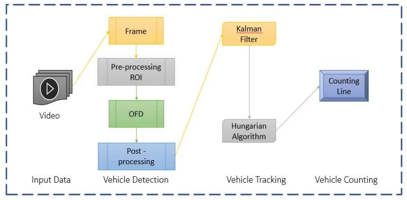
Research methodology framework
The proposed research method is divided into three main processes, including vehicle detection, vehicle tracking, and vehicle counting. The proposed research methodology framework is
1http://cvlab.aut.ac.ir/old/node/28.html
shown in Figure 1. Dataset video input is processed into a set of image frames with size (480 x 640). Preprocessing in this paper uses ROI polygon with sizes at points [220.0], [50,280], [600,280] and [430,0].
The vehicle detection process uses optical flow density which has been developed by OpenCV library using Farneback Algorithm. The Farneback method uses the base quadratic polynomial assumption. OpenCV gets a 2-channel array with optical flow vectors, (u, v). Next step is to find the magnitude and direction of flow vectors. Direction corresponds to Hue value of the image. Magnitude corresponds to Value plane. Image binarization is used to get the blob of vehicle object. The object of vehicles then optimized using dilation operation to connect the parts of an unbounded object or to close the hole in the object. Detection of vehicles objects in this paper using the segmentation of Contours from blob detection in the ROI region. Each vehicle object detected then find a centroid value by utilizing the moment feature. The centroid is used as position input for vehicle tracking using Hungarian Kalman filter.
The representation of objects on the Kalman filter using multivariate Gaussian assumptions. Mean (centroid) represents the existence of each object. While covariance represents uncertainty. Process noise and observation noise represent noise in the system.
𝑢 = [𝐶𝑥𝐶𝑦] (20)
The transition matrix represents the movement of an object by using the concept of linear displacement. The displacement is linearly represented by the movement of objects with fixed speed and minimal acceleration changes.
𝐹 = [ 1𝑑𝑡 𝑑𝑡1 ] (21)
Where 𝑑𝑡 is the time difference during the process of object displacement occurs. So based on the kalman filter equation, the state prediction from the previous input state is present in equation 22:
𝑢{′𝑘|𝑘 − 1} = 𝐹𝑢
{𝑘 − 1|𝑘 − 1}
′ (22)
[𝐶𝑥′𝐶𝑦′] = [𝑑𝑡 1 𝑑𝑡1 ] [𝐶𝑥𝐶𝑦] (23)
[𝑃𝑥′𝑃𝑦′] = [𝑑𝑡 1 𝑑𝑡1 ] [𝑃𝑥𝑃𝑦] [𝑑𝑡 1 𝑑𝑡1 ] 𝑑𝑡 + [𝑄𝑥𝑄𝑦] (25)
Q represents the noise process caused by the system's ability to detect blobs and camera quality capabilities. The prediction result of mean and covariance matrix is then corrected to update the position of the object by using observation result and Kalman gain. Kalman gain can be written mathematically with the equation 26
𝐾{𝑘} = 𝑃{𝑘|𝑘 − 1}𝐴. 𝑇(𝐶. 𝐼𝑛𝑣) (26)
Where A is a matrix that links the observation with the predicted result and C represents pre-fit residual covariance that can provide uncertainty information on observation noise.
𝐴 = [10 01] (27)
𝐶 = 𝐴𝑃{𝑘|𝑘 − 1}𝐴. 𝑇 + 𝑅 (28)
The equation 𝑏{𝑘} − 𝐴𝑢{′𝑘|𝑘 − 1}= 𝐵 is a
residual pre-fit measurement that can estimate and calculate the difference values between the actual measurements with the best predicted results available under the previous system model and measurement. The final result of updating the object position and uncertainty on the system can then be calculated using the equation 29 and 30. 𝑢{′𝑘|𝑘} = 𝑢
{𝑘|𝑘 − 1}
′ + 𝐾
{𝑘} 𝐵 (29)
𝑃{𝑘|𝑘} = 𝑃{𝑘|𝑘 − 1} − 𝐾{𝑘}(𝐶𝐾. 𝑇) (30) The Hungarian algorithm is an algorithm used
for assignment of two pairs of matrix inputs. Matrix input in this research is the distance between the object positions obtained from detection and prediction. The Hungarian Algorithm aims to create an optimal mapping for each component of the observed object [20]. The distance measurement parameter of the Hungarian algorithm used in this paper is a Euclidian distance such as equation 31:
d = √(Cxd−Cxkf)2+ (Cyd−Cykf)2 (31)
Where d is the distance, Cxd and Cyd are centroid values on the x and y-axes of detection using OFD, Cxkf and Cykf are centroid values on the x and y-axes of detection using KF.
Vehicles counting becomes one of the critical processes. Because the detection based counting has some weaknesses due to double and miscounting. This research uses single line counting which is placed at one specified frame location, 5/12 from frame width. In [2], counting line located according to the best results through trial and error. Changing the location of the counting line will affect the configuration of the development ITS system. In the video dataset, the occurrence of miss detection on a particular frame can cause a miscounting.
The measurement performances
To Evaluate our methods, we use six evaluation measurement performances. These are Percentage of correctly detected vehicles, falsely detected vehicles, correctly tracked vehicles, misses tracked vehicles, correctly counted vehicles, and falsely counted vehicles. Percentage of correctly detected vehicles is the ratio of the number of vehicles
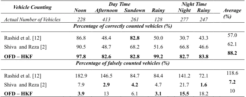
TABLE 3 VEHICLE COUNTING RESULT
Vehicle Counting Noon AfternoonDay TimeSundown Rainy NightNight TimeRainy Average (%)
Actual Number of Vehicles 228 413 261 128 277 247
Percentage of correctly counted vehicles (%)
Rashid et al. [12] 86.8 48.4 82.8 50.0 30.7 43.3 57.0
Shiva and Reza [2] 90.5 48.7 68.2 51.6 66.8 46.6 62.1
OFD – HKF 97.8 82.6 82.8 99.2 82.7 83.8 88.2
Percentage of falsely counted vehicles (%)
Rashid et al. [12] 182.9 146.5 84.7 84.4 141.2 72.1 118.6
Shiva and Reza [2] 7.9 2.9 4.2 4.7 21.7 1.6 7.2
detected and the number of vehicles matching ground truth multiplied by 100%; Percentage of falsely detected vehicles is the ratio of the number non-vehicle detected and the number of vehicles matching ground truth multiplied by 100%; Percentage of correctly tracked vehicles is the ratio of the number of successfully tracked vehicles and the number of vehicles matching ground truth multiplied by 100%; Percentage of misses tracked vehicles is the ratio of the number of untracked vehicles and the number of vehicles matching ground truth multiplied by 100%; Percentage of correctly counted vehicles is the ratio of the number of counted vehicles and the number of vehicles matching ground truth multiplied by 100%; and Percentage of falsely counted vehicles is the ratio of non-vehicle counted and the number of vehicles matching ground truth multiplied by 100%.
This research was tested on the Amirkabir dataset and compared with previous related studies [12] and [2]. The implementation algorithm conducted on laptop with specification Intel Core I5-6200U CPU @ 2.3 GHz 2.4 GHz with total RAM of 4 GB
3. Results and Analysis
Vehicle detection is the first step in research related to the development of intelligent traffic system (ITS). Further vehicle detection results can be utilized for tracking and counting the number of vehicles. Vehicle detection is the primary foundation for the development of high-quality
ITS. Detection of vehicles with good results will make ease to the next process. Therefore, vehicle detection becomes very important for developing the ITS. The dataset used consists of six data sets that have different characteristics. Each character has its challenges that must be addressed to avoid errors during object detection. Possible errors in object detection are miss detection and false detection. Miss detection object detection can occur due to differences in colour intensity between objects with the background while false detection can occur due to the movement of other objects such as shadows and emission of light from moving vehicles. Tables 1 shows the results of vehicle detection using Optical flow density method.
Table 1 shows the results of vehicle detection performance using Optical Flow Density (OFD) method compared with two previous research [12] and [2]. From table 1, it is known that the vehicle detection using optical flow density methods, implemented by the authors have an average accuracy 93.6%. Vehicle detection using optical flow density has a better result than [12]. [12] using TSI-VDL to detect the vehicles. Besides that, the proposed method shows the approach research to Shiva and Reza [2]. [2] use the ABM-SC method to detect the vehicles. The result of percentage false rate value shows the better result than [12] and [2]. The average value of false percentage rate is 1.2%. Vehicle verification use to minimize the false rate from this research. The parameters using the minimum contour area, length, and width of each bounding box size.
OFD has been implemented utilizing the features of gradient image. Vehicles detection using OFD in this paper was conducted to improve the performance of previous research, i.e. TSI-VDL [12] and ABM [2]. The implemented OFD method does not take much time to recognize the vehicles on the video dataset, compared with the TSI-VDL and ABM-SC methods. The TSI-VDL is only capable of detecting vehicles with an average accuracy performance only 57.0%.
Especially for night and afternoon datasets, the TSI-VDL [12] does not even achieve 50%. This is due to the movement of vehicle lights and shadow of vehicles. Also, the error rates using TSI-VDL method is also too high up to 118.6% on average. In table 1 the average accuracy performance of [2] reaching 98.2%. The vehicles detection result was obtained by taking five video frames from each dataset. Vehicles will be counted into detected vehicles if at least one frame detects the vehicle. This approach is not capable of detecting the vehicle at any frame.
The consistency of vehicle detection for each frame is one of the essential factors to be considered. This will be seen in the tracking and counting result. Regarding this issue, we use motion based appearance to detect the vehicle. So that the moving vehicle can be detected for every frame. Although the result is not as a good as ABM-SC. Vehicles are tracking in this paper using Hungarian Kalman filter algorithm. Hungarian Kalman filter is an algorithm used to track the object with the input of the previous object position.
Table 2 shows the results of vehicle tracking performance. The results of vehicle tracking performance were compared using two previous studies [12] and [2]. The Hungarian Kalman filter implemented in this paper performs better result than the previous methods. The average accuracy is 88.2%.
The Hungarian Kalman filter works well in the case of multi-object tracking. It can predict the position of objects in the future and associated data on each vehicle object. Tracking results using distance similarity measurement conducted by [2] have an average accuracy of 61.2%. The difference between vehicle detection and vehicle tracking performance showed the significant decrease from 98.2% to 61.2%.
In [12], the number of tracked vehicles is the number of detected vehicles. In this research, vehicle tracking and counting are determined by the particular id during vehicle detection. The performance of vehicles tracking is highly dependent on vehicle detection performance results. The accuracy performance from vehicles
tracking only 57% on average. The average performance of miss tracked using Hungarian Kalman filter method is 11.8%. This result is the best result compared to [2] and [12]. While the average performance of miss tracked by using the id detection based [12] and distance similarity measurement [2] reached 43% and 38% in average respectively. Miss tracked due to the occlusion problem so that adjacent vehicles are detected and tracked as one vehicle only. Moreover, the configuration of determining time and covariance matrix variables on the Kalman filter can also affect the results of object tracking. Time variable in this paper set as 0,025.
Vehicles are counting in this paper using single line counting (SLC) algorithm. SCL used to count the number of vehicles which have a small error rate [2].Table 3 shows the results of vehicle counting. Based on table 3, the proposed framework is the best method for vehicles counting. The developed framework has several advantages over the comparator. In [12], The accuracy performance obtained from this method only reached 57%. Some vehicles are mostly undetected. Same as vehicle tracking, due to double detection problems, so the error rate for vehicles is counting up to 118.6%. In [2], the accuracy performance below 70% in average, except for the Noon dataset. Although the location of the counting line was arranged based on the best trial and error. Visualization results for multi-object detection and tracking using OFD - HKF for vehicle counting shown in figure 2. Object centroid, counting line, and detected vehicles are visualized by using a red dot, blue line, and green bounding box, respectively. Trajectory tracking and the number of counted vehicles visualized using RGB and text “Number of Vehicles = n” in red colour randomly. Where “n” represents the number of counted vehicles.
4. Conclusion
the average value of a false rate for each process detection, tracking, and vehicle counting is 1.2%, 11.8% and 10.0% respectively.
References
[1] N. Kosaka and G. Ohashi, “Vision-Based Nighttime Vehicle Detection Using CenSurE and SVM,” IEEE Trans. Intell. Transp. Syst., vol. 16, no. 5, pp. 2599– 2608, 2015.
[2] S. Kamkar and R. Safabakhsh, “Vehicle detection, counting and classification in various conditions,” IET Intell. Transp. Syst., vol. 10, no. 6, pp. 406–413, 2016. [3] T. Chen and S. Lu, “Robust Vehicle
Detection and Viewpoint Estimation with Soft Discriminative Mixture Model,” IEEE Trans. Circuits Syst. Video Technol., vol. 27, no. 2, pp. 394–403, 2017. and G. Van Cutsem, “Optimising computer vision based ADAS: a vehicle detection case study,” IET Intell. Transp. Syst., vol. 10, no. 3, pp. 157–164, 2016.
[7] X. Wang, L. Xu, H. Sun, J. Xin, and N. Zheng, “On-Road Vehicle Detection and Tracking Using MMW Radar and Monovision Fusion,” IEEE Trans. Intell. Transp. Syst., vol. 17, no. 7, 2016. [8] J. M. Guo, C. H. Hsia, K. S. Wong, J. Y.
Wu, Y. T. Wu, and N. J. Wang, “Nighttime Vehicle Lamp Detection and Tracking with Adaptive Mask Training,” IEEE Trans. Veh. Technol., vol. 65, no. 6, 2016. [9] H. T. Chen, Y. C. Wu, and C. C. Hsu,
“Daytime Preceding Vehicle Brake Light Detection Using Monocular Vision,” IEEE Sens. J., vol. 16, no. 1, pp. 120–131, 2016. [10] S. Noh, D. Shim, and M. Jeon, “Adaptive Sliding-Window Strategy for Vehicle Detection in Highway Environments,” IEEE Trans. Intell. Transp. Syst., vol. 17, no. 2, pp. 323–335, 2016.
[11] Yi Wu and Jongwoo Lim and Ming-Hsuan Yang, “Online Object Tracking: A Benchmark” IEEE Conference on Computer Vision and Pattern Recognition (CVPR) 2013
[12] N. U. Rashid, N. C. Mithun, B. R. Joy, and S. M. M. Rahman, “Detection and
classification of vehicles from a video using a time-spatial image,” ICECE 2010 - 6th Int. Conf. Electr. Comput. Eng., no. December, pp. 502–505, 2010.
[13] Indrabayu, R. Y. Bakti, I. S. Areni, and A. A. Prayogi, “Vehicle detection and tracking using Gaussian Mixture Model and Kalman Filter,” Proc. - Cybern. 2016 Int. Conf. Comput. Intell. Cybern., 2017.
[14] A. Agarwal, S. Gupta, and D. K. Singh, “Review of optical flow technique for moving object detection,” Proc. 2016 2nd Int. Conf. Contemp. Comput. Informatics, IC3I 2016, pp. 409–413, 2016.
[15] S. Aslani and H. Mahdavi-nasab, “Optical Flow Based Moving Object Detection and Tracking for Traffic Surveillance,” vol. 7, no. 9, pp. 761–765, 2013.
[16] D. X. Zhou and H. Zhang, “Modified GMM Background Modeling and Optical Flow for Detection of Moving Objects,” 2005 IEEE Int. Conf. Syst. Man Cybern., vol. 3, no. December, pp. 2224–2229, 2005.
[17] K. Kale, S. Pawar, and P. Dhulekar, “Moving Object Tracking using Optical Flow and Motion Vector Estimation,” pp. 2– 7, 2015.
[18] E. Engineering, I. I. T. B. Mumbai, and I. I. T. B. Mumbai, “Dynamic Arbitrary Shape Boundary Detection and Tracking Using Hungarian Kalman Filter,” no. Boundary Detection, pp. 243–249, 2016.
[19] Z. Meng, Z. U. O. Yan, F. Y. Yu, and L. I. M. Di, “Sensor Assignment Method Based on Time-Varying Measurement Variance for Tracking Multi-targets,” no. 1, pp. 3368– 3372, 2016.
[20] B. Sahbani and W. Adiprawita, “Kalman Filter and Iterative-Hungarian Algorithm Implementation for Low Complexity Point Tracking as Part of Fast Multiple Object Tracking System,” 6th Int. Conf. Syst. Eng. Technol., pp. 109–115, 2016.
[21] R. O’Malley, E. Jones, and M. Glavin, “Rear-lamp vehicle detection and tracking in the low-exposure colour video for night conditions,” IEEE Trans. Intell. Transp. Syst., vol. 11, no. 2, pp. 453–462, 2010. [22] R. O’Malley, M. Glavin, and E. Jones,
“Vision-based detection and tracking of vehicles to the rear with perspective correction in low-light conditions,” IET Intell. Transp. Syst., vol. 5, no. 1, pp. 1–10, 2011.