Chaos Theory Tamed
Garnett P. Williams US Geological Survey (Ret.)
JOSEPH HENRY PRESS
2101 Constitution Avenue, NW Washington, DC 20418
The JOSEPH HENRY PRESS, an imprint of the NATIONAL ACADEMY PRESS, was created by the National Academy of Sciences and its affiliated institutions with the goal of making books on science, technology, and health more widely available to professionals and the public. Joseph Henry was one of the founders of the National Academy of Sciences and a leader of early American science.
Any opinions, findings, conclusions, or recommendations expressed in this volume are those of the author and do not necessarily reflect the views of the National Academy of Sciences or its affiliated institutions.
Library of Congress Catalog Card Number 97-73862 International Standard Book Number 0-309-06351-5
Additional copies of this book are available from:
JOSEPH HENRY PRESS/NATIONAL ACADEMY PRESS 2101 Constitution Avenue, NW
Washington, DC 20418 1-800-624-6242 (phone)
1-202-334-3313 (phone in Washington DC) 1-202-334-2451 (fax)
Visit our Web site to read and order books on-line: http://www.nap.edu
Copyright © 1997 Garnett P. Williams. All rights reserved. Published by arrangement with Taylor & Francis Ltd.
Reprinted 1999
PREFACE
Virtually every branch of the sciences, engineering, economics, and related fields now discusses or refers to chaos. James Gleick's 1987 book, Chaos: making a new science and a 1988 one-hour television program on chaos aroused many people's curiosity and interest. There are now quite a few books on the subject. Anyone writing yet another book, on any topic, inevitably goes through the routine of justifying it. My justification consists of two reasons:
• Most books on chaos, while praiseworthy in many respects, use a high level of math. Those books have been written by specialists for other specialists, even though the authors often label them "introductory." Amato (1992) refers to a "cultural chasm" between "the small group of mathematically inclined initiates who have been touting" chaos theory, on the one hand, and most scientists (and, I might add, "everybody else''), on the other. There are relatively few books for those who lack a strong mathematics and physics background and who might wish to explore chaos in a particular field. (More about this later in the Preface.)
• Most books, in my opinion, don't provide understandable derivations or explanations of many key concepts, such as Kolmogorov-Sinai entropy, dimensions, Fourier analysis, Lyapunov exponents, and others. At present, the best way to get such explanations is either to find a personal guru or to put in gobs of frustrating work studying the brief, condensed, advanced treatments given in technical articles.
Chaos is a mathematical subject and therefore isn't for everybody. However, to understand the fundamental concepts, you don't need a background of anything more than introductory courses in algebra, trigonometry, geometry, and statistics. That's as much as you'll need for this book. (More advanced work, on the other hand, does require integral calculus, partial differential equations, computer programming, and similar topics.)
In this book, I assume no prior knowledge of chaos, on your part. Although chaos covers a broad range of topics, I try to discuss only the most important ones. I present them hierarchically. Introductory background perspective takes up the first two chapters. Then come seven chapters consisting of selected important material (an auxiliary toolkit) from various fields. Those chapters provide what I think is a good and necessary
foundation—one that can be arduous and time consuming to get from other sources. Basic and simple chaos-related concepts follow. They, in turn, are prerequisites for the slightly more advanced concepts that make up the later chapters. (That progression means, in turn, that some chapters are on a very simple level, others on a more advanced level.) In general, I try to present a plain-vanilla treatment, with emphasis on the idealized case of low-dimensional, noise-free chaos. That case is indispensable for an introduction. Some real-world data, in contrast, often require sophisticated and as-yet-developing methods of analysis. I don't discuss those techniques. The absence of high-level math of course doesn't mean that the reading is light entertainment. Although there's no way to avoid some specialized terminology, I define such terms in the text as well as in a Glossary. Besides, learning and using a new vocabulary (a new language) is fun and exciting. It opens up a new world.
I'm a geologist/hydrologist by training. I believe that coming from a peripheral field helps me to see the subject differently. It also helps me to understand—and I hope answer—the types of questions a nonspecialist has. Finally, I hope it will help me to avoid using excessive amounts of specialized jargon.
In a nutshell, this is an elementary approach designed to save you time and trouble in acquiring many of the fundamentals of chaos theory. It's the book that I wish had been available when I started looking into chaos. I hope it'll be of help to you.
In regard to units of measurement, I have tried to compromise between what I'm used to and what I suspect most readers are used to. I've used metric units (kilometers, centimeters, etc.) for length because that's what I have always used in the scientific field. I've used Imperial units (pounds, Fahrenheit, etc.) in most other cases.
I sincerely appreciate the benefit of useful conversations with and/or help from A. V. Vecchia, Brent Troutman, Andrew Fraser, Ben Mesander, Michael Mundt, Jon Nese, William Schaffer, Randy Parker, Michael Karlinger, Leonard Smith, Kaj Williams, Surja Sharma, Robert Devaney, Franklin Horowitz, and John Moody. For
critically reading parts of the manuscript, I thank James Doerer, Jon Nese, Ron Charpentier, Brent Troutman, A. V. Vecchia, Michael Karlinger, Chris Barton, Andrew Fraser, Troy Shinbrot, Daniel Kaplan, Steve Pruess, David Furbish, Liz Bradley, Bill Briggs, Dean Prichard, Neil Gershenfeld, Bob Devaney, Anastasios Tsonis, and Mitchell Feigenbaum. Their constructive comments helped reduce errors and bring about a much more readable and understandable product. I also thank Anthony Sanchez, Kerstin Williams, and Sebastian Kuzminsky for their invaluable help on the figures.
SYMBOLS
(a) A constant; (b) a component dimension in deriving the Hausdorff-Besicovich dimension
ca
Intercept of line ∆R=ca-H'KSm,and taken as a rough indicator of the accuracy of the measurements
d
Component dimension in deriving Hausdorff-Besicovich dimension; elsewhere, a derivative
e
Base of natural logarithms, with a value equal to 2.718. . .
f
A function
h
Harmonic number
i
A global counter, often representing the ith bin of the group of bins into which we divide values of x
j
(a) A counter, often representing the jth bin of the group of bins into which we divide values of y; (b) the imaginary number (-1)0.5
k value (logistic equation) at which chaos begins
m
A chosen lag, offset, displacement, or number of intervals between points or observations
n
Number (position) of an iteration, observation or period within a sequence (e.g. the nth observation)
r
Scaling ratio
s
s2
Variance (same as power)
t
Time, sometimes measured in actual units and sometimes just in numbers of events (no units)
u
A trajectory point to which distances from point xiare measured in calculating the correlation dimension
xn
Height of the wave having harmonic number h
y0
Value of dependent variable y at the origin
z
Dc
Capacity (a type of dimension)
DH
Hausdorff (or Hausdorff-Besicovich) dimension
DI
Information dimension, numerically equal to the slope of a straight line on a plot of Iε (arithmetic scale) versus
1/ε (log scale)
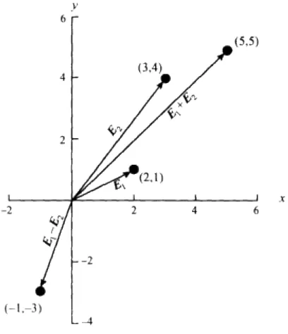
E
An observed vector, usually not perpendicular to any other observed vectors
F
Entropy computed as a weighted sum of the entropies of individual phase space compartments
HKS
Kolmogorov-Sinai (K-S) entropy
H'KS
Kolmogorov-Sinai (K-S) entropy as estimated from incremental redundancies
HX
Entropy computed over a particular duration of time t
I
Ii
Mutual information of coupled systemsXand Y
IY
Information of dynamical system Y
IY;X
Mutual information of coupled systemsXand Y
Iε
Information needed to describe an attractor or trajectory to within an accuracy ε
K
Boltzmann's constant
L
Length or distance
Lε
Estimated length, usually by approximations with small, straight increments of length ε
Lw
Wavelength
Mε
An estimate of a measure (a determination of length, area, volume, etc.)
Mtr
Total number of possible bin-routes a dynamical system can take during its evolution from an arbitrary starting time to some later time
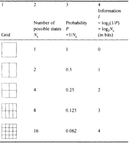
Ns
Total number of possible or represented states of a system Νε
P
Probability
Pi
(a) Probability associated with the ith box, sphere, value, etc.; (b) all probabilities of a distribution, as a group
Ps
Sequence probability
P(xi)
(a) Probability of class xi from system X; (b) all probabilities of the various classes of x, as a group
P(xi,yj)
Joint probability that system x is in class xiwhen system Y is in class yj
P(yj)
(a) Probability of class yj from system Y; (b) all probabilities of the various classes of y,as a group
P(yj|xi)
Conditional probability that system Y will be in class yj, given that systemXis in class xi
R
A unit vector representing any of a set of mutually orthogonal vectors
V
A vector constructed from an observed vector so as to be orthogonal to similarly constructed vectors of the same set
X
A system or ensemble of values of random variable x and its probability distribution
Y
A system or ensemble of values of random variable y and its probability distribution
α
Fourier cosine coefficient
ß
Fourier sine coefficient
δ
δa
Orbit difference obtained by extrapolating a straight line back to n=0 on a plot of orbit difference versus iteration n
δ0
Difference between starting values of two trajectories
ε
Characteristic length of scaling device (ruler, box, sphere, etc.)
ε0
Largest length of scaling device for which a particular relation holds
θ
(a) Central or inclusive angle, such as the angle subtended during a rotating-disk experiment (excluding phase angle) or the angle between two vectors: (b) an angular variable or parameter
λ
Lyapunov exponent (global, not local)
ν
Correlation dimension (correlation exponent)
Estimated correlation dimension
π
3.1416. . .
φ
phase angle
Σ
summation symbol
∆
an interval, range, or difference
∆R
incremental redundancy (redundancy at a given lag minus redundancy at the previous lag)
|
PART I
BACKGROUND
Chapter 1
Introduction
The concept of chaos is one of the most exciting and rapidly expanding research topics of recent decades. Ordinarily, chaos is disorder or confusion. In the scientific sense, chaos does involve some disarray, but there's much more to it than that. We'll arrive at a more complete definition in the next chapter.
The chaos that we'll study is a particular class of how something changes over time.In fact, change and time are the two fundamental subjects that together make up the foundation of chaos. The weather, Dow-Jones industrial average, food prices, and the size of insect populations, for example, all change with time. (In chaos jargon, these are called systems.A "system" is an assemblage of interacting parts, such as a weather system.
Alternatively, it is a group or sequence of elements, especially in the form of a chronologically ordered set of data. We'll have to start speaking in terms of systems from now on.) Basic questions that led to the discovery of chaos are based on change and time. For instance, what's the qualitative long-term behavior of a changing system? Or, given nothing more than a record of how something has changed over time, how much can we learn about the underlying system? Thus, "behavior over time" will be our theme.
The next chapter goes over some reasons why chaos can be important to you. Briefly, if you work with
numerical measurements (data), chaos can be important because its presence means that long-term predictions are worthless and futile. Chaos also helps explain irregular behavior of something over time. Finally, whatever your field, it pays to be familiar with new directions and new interdisciplinary topics (such as chaos) that play a prominent role in many subject areas. (And, by the way, the only kind of data we can analyze for chaos are rankable numbers, with clear intervals and a zero point as a standard. Thus, data such as "low, medium, or high" or "male/female" don't qualify.)
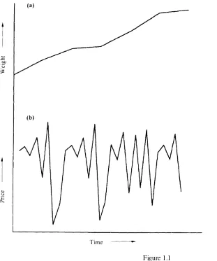
Figure 1.1
Hypothetical time series: (a) change of a baby's weight with time; (b) change in price of wheat over time.
Even when people don't have any numerical measurements, they can simulate a time series using some specified rule, usually a mathematical equation. The equation describes how a quantity changes from some known
beginning state. Figure 1.1b—a pattern that happens to be chaotic—is an example. I generated the pattern with the following special but simple equation (from Grebogi et al. 1983):
xt + 1 = 1.9-xt2 (1.1)
Here xt (spoken as "x of t")is the value of x at a time t, and xt+1 ("x of t plus one") is the value of x at some time
interval (day, year, century, etc.) later. That shows one of the requirements for chaos: the value at any time depends in part on the previous value. (The price of a loaf of bread today isn't just a number pulled out of a hat; instead, it depends largely on yesterday's price.) To generate a chaotic time series with Equation 1.1, I first assigned (arbitrarily) the value 1.0 for xtand used the equation to compute xt+1. That gave xt+1=1.9-12=0.9. To
simulate the idea that the next value depends on the previous one, I then fed back into the equation the xt+1 just
computed (0.9), but put it in the position of the given xt.Solving for the new xt+1 gave xt+1=1.9-0.92=1.09. (And so
time here is represented by repeated calculations of the equation.) For the next time increment, the computed xt+1
Input value (xt) New value (xt+1)
Repeating this process about 30 times produced a record of widely fluctuating values of xt+1 (the time series of
Figure 1. 1b).
Just looking at the time series of Figure 1.1b, nobody can tell whether it is chaotic. In other words, erratic-looking temporal behavior is just a superficial indicator of possible chaos. Only a detailed analysis of the data, as explained in later chapters, can reveal whether the time series is chaotic.
The simulated time series of Figure 1.1b has several key traits:
• It shows complex, unsystematic motion (including large, sudden qualitative changes), rather than some simple curve, trend, cycle, or equilibrium. (A possible analogy is that many evolving systems in our world show instability, upheaval, surprise, perpetual novelty, and radical events.)
• The indiscriminate-looking pattern didn't come from a haphazard process, such as plucking numbered balls out of a bowl. Quite the contrary: it came from a specific equation. Thus, a chaotic sequence looks haphazard but really is deterministic,meaning that it follows a rule. That is, some law, equation, or fixed procedure determines or specifies the results. Furthermore, for given values of the constants and input, future results are predictable. For instance, given the constant 1.9 and a value for xtin Equation 1.1, we can
compute xt+1 exactly. (Because of that deterministic origin, some people refer to chaos as "deterministic
chaos.")
• The equation that generated the chaotic behavior (Eq. 1.1) is simple. Therefore, complex behavior doesn't necessarily have a complex origin.
• The chaotic behavior came about with just one variable (x). (A variable is a quantity that can have different numerical values.) That is, chaos doesn't have to come from the interaction of many variables. Instead, just one variable can do it.
• The pattern is entirely self-generated. In other words, aside from any influence of the constant (explored in later chapters), the chaos develops without any external influences whatsoever.
• The irregular evolution came about without the direct influence of sampling or measurement error in the calculations. (There aren't any error terms in the equation.)
The revelation that disorganized and complex-looking behavior can come from an elementary, deterministic equation or simple underlying cause was a real surprise to many scientists. Curiously, various fields of study many years earlier accepted a related idea: collections of small entities (particles or whatever) behave
Equation 1.1 shows why many scientists are attracted to chaos: behavior that looks complex and even
impossible to decipher and understand can be relatively easy and comprehensible. Another attraction for many of us is that many basic concepts of chaos don't require advanced mathematics, such as calculus, differential equations, complex variables, and so on. Instead, you can grasp much of the subject with nothing more than basic algebra, plane geometry, and maybe some rudimentary statistics. Finally, an unexpected and welcome blessing is that, to analyze for chaos, we don't have to know the underlying equation or equations that govern the system.
Chaos is a young and rapidly developing field. Indeed, much of the information in this book was only
discovered since the early 1970s. As a result, many aspects of chaos are far from understood or resolved. The most important unresolved matter is probably this: at present, chaos is extremely difficult to identify in
real-world data.It certainly appears in mathematical (computer) exercises and in some laboratory experiments. (In
fact, as we'll see later, once we introduce the idea of nonlinearity into theoretical models, chaos is unavoidable.) However, there's presently a big debate as to whether anyone has clearly identified chaos in field data. (The same difficulty, of course, accompanies the search for any kind of complex structure in field data. Simple patterns we can find and approximate; complex patterns are another matter.) In any event, we can't just grab a nice little set of data, apply a simple test or two, and declare "chaos" or "no chaos."
The reason why recognizing chaos in real-world data is such a monumental challenge is that the analysis methods aren't yet perfected. The tools we have right now look attractive and enticing. However, they were developed for highly idealized conditions, namely:
• systems of no more than two or three variables
• very big datasets (typically many thousands of observations,and in some cases millions)
• unrealistically high accuracy in the data measurements
• data having negligible amounts of noise (unwanted disturbance superimposed on, or unexplainable variability in, useful data).
Problems arise when data don't fulfil those four criteria. Ordinary data (mine and very possibly yours) rarely fulfil them. For instance, datasets of 50-100 values (the kind I'm used to) are way too small. One of the biggest problems is that, when applied to ordinary data, the present methods often give plausible but misleading results, suggesting chaos when in fact there isn't any.
Having said all that, here's something equally important on the positive side: applying chaos analysis to a set of data (even if those data aren't ideal) can reveal many important features that other, more traditional tools might not disclose.
Description and theory of chaos are far ahead of identifying chaos in real-world data. However, with the present popularity of chaos as a research topic, new and improved methods are emerging regularly.
Summary
Chapter 2
Chaos in perspective
Where Chaos Occurs
Chaos, as mentioned, deals mostly with how something evolves over time. Space or distance can take the place of time in many instances. For that reason, some people distinguish between ''temporal chaos" and "spatial chaos."
What kinds of processes in the world are susceptible to chaos? Briefly, chaos happens only in deterministic,
nonlinear, dynamical systems. (I'll define "nonlinear" and "dynamical" next. At the end of the book there is a glossary of these and other important terms.) Based on those qualifications, here's an admittedly imperfect but nonetheless reasonable definition of chaos:
Chaos is sustained and disorderly-looking long-term evolution that satisfies certain special mathematical criteria and that occurs in a deterministic nonlinear system.
Chaos theory is the principles and mathematical operations underlying chaos.
Nonlinearity
Nonlinear means that output isn't directly proportional to input, or that a change in one variable doesn't produce
a proportional change or reaction in the related variable(s). In other words, a system's values at one time aren't proportional to the values at an earlier time. An alternate and sort of "cop-out" definition is that nonlinear refers to anything that isn't linear, as defined below. There are more formal, rigid, and complex mathematical
definitions, but we won't need such detail. (In fact, although the meaning of "nonlinear" is clear intuitively, the experts haven't yet come up with an all-inclusive definition acceptable to everyone. Interestingly, the same is true of other common mathematical terms, such as number, system, set, point, infinity, random, and certainly chaos.) A nonlinear equation is an equation involving two variables, say x and y, and two coefficients,say b and c, in some form that doesn't plot as a straight line on ordinary graph paper.
The simplest nonlinear response is an all-or-nothing response, such as the freezing of water. At temperatures higher than 0°C, nothing happens. At or below that threshold temperature, water freezes. With many other examples, a nonlinear relation describes a curve, as opposed to a threshold or straight-line relation, on arithmetic (uniformly scaled) graph paper.
Most of us feel a bit uncomfortable with nonlinear equations. We prefer a linear relation any time. A linear
equation has the form y=c+bx. It plots as a straight line on ordinary graph paper. Alternatively, it is an
equation in which the variables are directly proportional, meaning that no variable is raised to a power other than one. Some of the reasons why a linear relation is attractive are:
• the equation is easy
• we're much more familiar and comfortable with the equation
• extrapolation of the line is simple
• comparison with other linear relations is easy and understandable
Classical mathematics wasn't able to analyze nonlinearity effectively, so linear approximations to curves became standard. Most people have such a strong preference for straight lines that they usually try to make nonlinear relations into straight lines by transforming the data (e.g. by taking logarithms of the data). (To "transform"data means to change their numerical description or scale of measurement.) However, that's mostly a graphical or analytical convenience or gimmick. It doesn't alter the basic nonlinearity of the physical process. Even when people don't transform the data, they often fit a straight line to points that really plot as a curve. They do so because either they don't realize it is a curve or they are willing to accept a linear
approximation.
Campbell (1989) mentions three ways in which linear and nonlinear phenomena differ from one another:
• Behavior over time Linear processes are smooth and regular, whereas nonlinear ones may be regular at
first but often change to erratic-looking.
• Response to small changes in the environment or to stimuli A linear process changes smoothly and in
proportion to the stimulus; in contrast, the response of a nonlinear system is often much greater than the stimulus.
• Persistence of local pulses Pulses in linear systems decay and may even die out over time. In nonlinear systems, on the other hand, they can be highly coherent and can persist for long times, perhaps forever.
A quick look around, indoors and out, is enough to show that Nature doesn't produce straight lines. In the same way, processes don't seem to be linear. These days, voices are firmly declaring that many—possibly
most—actions that last over time are nonlinear. Murray (1991), for example, states that "If a mathematical model for any biological phenomenon is linear, it is almost certainly irrelevant from a biological viewpoint." Fokas (1991) says: "The laws that govern most of the phenomena that can be studied by the physical sciences, engineering, and social sciences are, of course, nonlinear." Fisher (1985) comments that nonlinear motions make up by far the most common class of things in the universe. Briggs & Peat (1989) say that linear systems seem almost the exception rather than the rule and refer to an "ever-sharpening picture of universal
nonlinearity." Even more radically, Morrison (1988) says simply that "linear systems don't exist in nature." Campbell et al. (1985) even object to the term nonlinear, since it implies that linear relations are the norm or standard, to which we're supposed to compare other types of relations. They attribute to Stanislaw Ulam the comment that using the term "nonlinear science" is like referring to the bulk of zoology as the study of non-elephant animals.
Dynamics
The word dynamics implies force, energy, motion, or change. A dynamical system is anything that moves, changes, or evolves in time. Hence, chaos deals with what the experts like to refer to as dynamical-systems
theory (the study of phenomena that vary with time) or nonlinear dynamics (the study of nonlinear movement
or evolution).
Motion and change go on all around us, every day. Regardless of our particular specialty, we're often interested in understanding that motion. We'd also like to forecast how something will behave over the long run and its eventual outcome.
Dynamical systems fall into one of two categories, depending on whether the system loses energy. A
conservative dynamical system has no friction; it doesn't lose energy over time. In contrast, a dissipative
Phenomena happen over time in either of two ways. One way is at discrete (separate or distinct) intervals. Examples are the occurrence of earthquakes, rainstorms, and volcanic eruptions. The other way is continuously
(air temperature and humidity, the flow of water in perennial rivers, etc.). Discrete intervals can be spaced evenly in time, as implied for the calculations done for Figure 1.1b, or irregularly in time. Continuous phenomena might be measured continuously, for instance by the trace of a pen on a slowly moving strip of paper. Alternatively, we might measure them at discrete intervals. For example, we might measure air temperature only once per hour, over many days or years.
Special types of equations apply to each of those two ways in which phenomena happen over time. Equations for discrete time changes are difference equations and are solved by iteration,explained below. In contrast, equations based on a continuous change (continuous measurements) are differential equations.
You'll often see the term "flow" with differential equations. To some authors (e.g. Bergé et al. 1984: 63), a flow is a system of differential equations. To others (e.g. Rasband 1990: 86), a flow is the solution of differential equations.
Differential equations are often the most accurate mathematical way to describe a smooth continuous evolution. However, some of those equations are difficult or impossible to solve. In contrast, difference equations usually can be solved right away. Furthermore, they are often acceptable approximations of differential equations. For example, a baby's growth is continuous, but measurements taken at intervals can approximate it quite well. That is, it is a continuous development that we can adequately represent and conveniently analyze on a discrete-time basis. In fact, Olsen & Degn (1985) say that difference equations are the most powerful vehicle to the
understanding of chaos. We're going to confine ourselves just to discrete observations in this book. The physical process underlying those discrete observations might be discrete or continuous.
Iteration is a mathematical way of simulating discrete-time evolution. To iterate means to repeat an operation over and over. In chaos, it usually means to solve or apply the same equation repeatedly, often with the outcome of one solution fed back in as input for the next, as we did in Chapter 1 with Equation 1.1. It is a standard method for analyzing activities that take place in equal, discrete time steps or continuously, but whose equations can't be solved exactly, so that we have to settle for successive discrete approximations (e.g. the time-behavior of materials and fluids). I'll use "number of iterations" and "time" synonymously and interchangeably from now onward.
Iteration is the mathematical counterpart of feedback.Feedback in general is any response to something sent out. In mathematics, that translates as "what goes out comes back in again." It is output that returns to serve as input. In temporal processes, feedback is that part of the past that influences the present, or that part of the present that influences the future. Positive feedback amplifies or accelerates the output. It causes an event to become magnified over time. Negative feedback dampens or inhibits output, or causes an event to die away over time. Feedback shows up in climate, biology, electrical engineering, and probably in most other fields in which processes continue over time.
The time frame over which chaos might occur can be as short as a fraction of a second. At the other extreme, the time series can last over hundreds of thousands of years, such as from the Pleistocene Epoch (say about 600000 years ago) to the present.
In theory, virtually anything that happens over time could be chaotic. Examples are epidemics, pollen production, populations, incidence of forest fires or droughts, economic changes, world ice volume, rainfall rates or amounts, and so on. People have looked for (or studied) chaos in physics, mathematics,
communications, chemistry, biology, physiology, medicine, ecology, hydraulics, geology, engineering, atmospheric sciences, oceanography, astronomy, the solar system, sociology, literature, economics, history, international relations, and in other fields. That makes it truly interdisciplinary. It forms a common ground or builds bridges between different fields of study.
Uncertain prominence
Opinions vary widely as to the importance of chaos in the real world. At one extreme are those scientists who dismiss chaos as nothing more than a mathematical curiosity. A middle group is at least receptive. Conservative members of the middle group feel that chaos may well be real but that the evidence so far is more illusory than scientific (e.g. Berryman & Millstein 1989). They might say, on the one hand, that chaos has a rightful place as a study topic and perhaps ought to be included in college courses (as indeed it is). On the other hand, they feel that it doesn't necessarily pervade everything in the world and that its relevance is probably being oversold. This sizeable group (including many chaos specialists) presently holds that, although chaos appears in mathematical experiments (iterations of nonlinear equations) and in tightly controlled laboratory studies, nobody has yet conclusively found it in the physical world.
Moving the rest of the way across the spectrum of attitudes brings us to the exuberant, ecstatic fringe element. That euphoric group holds that chaos is the third scientific revolution of the twentieth century, ranking right up there with relativity and quantum mechanics. Such opinions probably stem from reports that researchers find or claim to find chaos in chemical reactions, the weather, asteroid movement, the motion of atoms held in an electromagnetic field, lasers, the electrical activity of the heart and brain, population fluctuations of plants and animals, the stock market, and even in the cries of newborn babies (Pool 1989a, Mende et al. 1990). One enthusiastic proponent believes there's now substantial though non-rigorous evidence that chaos is the rule rather than the exception in Newtonian dynamics. He also says that "few observers doubt that chaos is ubiquitous throughout nature" (Ford 1989). Verification or disproval of such a claim awaits further research.
Causes Of Chaos
Chaos, as Chapter 1 showed, can arise simply by iterating mathematical equations. Chapter 13 discusses some factors that might cause chaos in such iterations.
The conditions required for chaos in our physical world (Bergé et al. 1984: 265), on the other hand, aren't yet fully known. In other words, if chaos does develop in Nature, the reason generally isn't clear. Three possible causes have been proposed:
• An increase in a control factor to a value high enough that chaotic, disorderly behavior sets in. Purely mathematical calculations and controlled laboratory experiments show this method of initiating chaos. Examples are iterations of equations of various sorts, the selective heating of fluids in small containers (known as Rayleigh-Benard experiments), and oscillating chemical reactions (Belousov-Zhabotinsky
experiments). Maybe that same cause operates with natural physical systems out in the real world (or maybe it doesn't). Berryman & Millstein (1989), for example, believe that even though natural ecosystems
• The nonlinear interaction of two or more separate physical operations. A popular classroom example is the double pendulum—one pendulum dangling from the lower end of another pendulum, constrained to move in a plane. By regulating the upper pendulum, the teacher makes the lower pendulum flip about in strikingly chaotic fashion.
• The effect of ever-present environmental noise on otherwise regular motion (Wolf 1983). At the least, such noise definitely hampers our ability to analyze a time series for chaos.
Benefits of Analyzing for Chaos
Important reasons for analyzing a set of data for chaos are:
• Analyzing data for chaos can help indicate whether haphazard-looking fluctuations actually represent an orderly system in disguise. If the sequence is chaotic, there's a discoverable law involved, and a promise of greater understanding.
• Identifying chaos can lead to greater accuracy in short-term predictions. Farmer & Sidorowich (1988a) say that "most forecasting is currently done with linear methods. Linear dynamics cannot produce chaos, and linear methods cannot produce good forecasts for chaotic time series." Combining the principles of chaos, including nonlinear methods, Farmer & Sidorowich found that their forecasts for short time periods were roughly 50 times more accurate than those obtained using standard linear methods.
• Chaos analysis can reveal the time-limits of reliable predictions and can identify conditions where long-term forecasting is largely meaningless. If something is chaotic, knowing when reliable predictability dies out is useful, because predictions for all later times are useless. As James Yorke said, "it's worthwhile knowing ahead of time when you can't predict something" (Peterson 1988).
• Recognizing chaos makes modeling easier. (A model is a simplified representation of some process or phenomenon. Physical or scale models are miniature replicas [e.g. model airplanes] of something in real life. Mathematical or statistical models explain a process in terms of equations or statistics. Analog models simulate a process or system by using one-to-one "analogous" physical quantities [e.g. lengths, areas, ohms, or volts] of another system. Finally, conceptual models are qualitative sketches or mental images of how a process works.) People often attribute irregular evolution to the effects of many external factors or variables. They try to model that evolution statistically (mathematically). On the other hand, just a few variables or deterministic equations can describe chaos.
Although chaos theory does provide the advantages just mentioned, it doesn't do everything. One area where it is weak is in revealing details of a particular underlying physical law or governing equation. There are instances where it might do so (see, for example, Farmer & Sidorowich 1987, 1988a, b, Casdagli 1989, and Rowlands & Sprott 1992). At present, however, we usually don't look for (or expect to discover) the rules by which a system evolves when analyzing for chaos.
Contributions of Chaos Theory
Some important general benefits or contributions from the discovery and development of chaos theory are the following.
Realizing that a simple, deterministic equation can create a highly irregular or unsystematic time series has forced us to reconsider and revise the long-held idea of a clear separation between determinism and
randomness. To explain that, we've got to look at what "random"means. Briefly, there isn't any general
agreement. Most people think of "random" as disorganized, haphazard, or lacking any apparent order or pattern. However, there's a little problem with that outlook: a long list of random events can show streaks, clumps, or patterns (Paulos 1990: 59-65). Although the individual events are not predictable, certain aspects of the clumps are.
Other common definitions of "random" are:
• every possible value has an equal chance of selection
• a given observation isn't likely to recur
• any subsequent observation is unpredictable
• any or all of the observations are hard to compute (Wegman 1988).
My definition, modified from that of Tashman & Lamborn (1979: 216) is: random means based strictly on a chance mechanism (the luck of the draw), with negligible deterministic effects. That definition implies that, in spite of what most people probably would assume, anything that is random really has some inherent
determinism, however small. Even a flip of a coin varies according to some influence or associated forces. A strong case can be made that there isn't any such thing as true randomness, in the sense of no underlying determinism or outside influence (Ford 1983, Kac 1983, Wegman 1988). In other words, the two terms
"random" and "deterministic" aren't mutually exclusive; anything random is also deterministic, and both terms can characterize the same sequence of data. That notion also means that there are degrees of randomness (Wegman 1988). In my usage, "random" implies negligible determinism.
People used to attribute apparent randomness to the interaction of complex processes or to the effects of external unmeasured forces. They routinely analyzed the data statistically. Chaos theory shows that such behavior can be attributable to the nonlinear nature of the system rather than to other causes.
Dynamical systems technology
Recognition and study of chaos has fostered a whole new technology of dynamical systems. The technology collectively includes many new and better techniques and tools in nonlinear dynamics, time-series analysis, short- and long-range prediction, quantifying complex behavior, and numerically characterizing non-Euclidean objects. In other words, studying chaos has developed procedures that apply to many kinds of complex systems, not just chaotic ones. As a result, chaos theory lets us describe, analyze, and interpret temporal data (whether chaotic or not) in new, different, and often better ways.
Nonlinear dynamical systems
Controlling chaos
Studying chaos has revealed circumstances under which we might want to avoid chaos, guide a system out of it, design a product or system to lead into or against it, stabilize or control it, encourage or enhance it, or even exploit it. Researchers are actively pursuing those goals. For example, there's already a vast literature on controlling chaos (see, for instance, Abarbanel et al. 1993, Shinbrot 1993, Shinbrot et al. 1993, anonymous 1994). Berryman (1991) lists ideas for avoiding chaos in ecology. A field where we might want to encourage chaos is physiology; studies of diseases, nervous disorders, mental depression, the brain, and the heart suggest that many physiological features behave chaotically in healthy individuals and more regularly in unhealthy ones (McAuliffe 1990). Chaos reportedly brings about greater efficiency in mixing processes (Pool 1990b, Ottino et al. 1992). Finally, it might help encode electronic messages (Ditto & Pecora 1993).
Historical Development
The word "chaos" goes back to Greek mythology, where it had two meanings:
• the primeval emptiness of the universe before things came into being
• the abyss of the underworld.
Later it referred to the original state of things. In religion it has had many different and ambiguous meanings over many centuries. Today in everyday English it usually means a condition of utter confusion, totally lacking in order or organization. Robert May (1974) seems to have provided the first written use of the word in regard to deterministic nonlinear behavior, but he credits James Yorke with having coined the term.
Foundations
Various bits and snatches of what constitutes deterministic chaos appeared in scientific and mathematical literature at least as far back as the nineteenth century. Take, for example, the chaos themes of sensitivity to
initial conditions and long-term unpredictability. The famous British physicist James Clerk Maxwell reportedly
said in an 1873 address that ". . .When an infinitely small variation in the present state may bring about a finite difference in the state of the system in a finite time, the condition of the system is said to be unstable . . . [and] renders impossible the prediction of future events, if our knowledge of the present state is only approximate, and not accurate" (Hunt & Yorke 1993). French mathematician Jacques Hadamard remarked in an 1898 paper that an error or discrepancy in initial conditions can render a system's long-term behavior unpredictable (Ruelle 1991: 47-9). Ruelle says further that Hadamard's point was discussed in 1906 by French physicist Pierre
Duhem, who called such long-term predictions "forever unusable." In 1908, French mathematician, physicist, and philosopher Henri Poincaré contributed a discussion along similar lines. He emphasized that slight differences in initial conditions eventually can lead to large differences, making prediction for all practical purposes "impossible." After the early 1900s the general theme of sensitivity to initial conditions receded from attention until Edward Lorenz's work of the 1960s, reviewed below.
During the twentieth century many mathematicians and scientists contributed parts of today's chaos theory. Jackson (1991) and Tufillaro et al. (1992: 323-6) give good skeletal reviews of key historical advances. May (1987) and Stewart (1989a: 269) state, without giving details, that some biologists came upon chaos in the 1950s. However, today's keen interest in chaos stems largely from a 1963 paper by meteorologist Edward Lorenz1 of the Massachusetts Institute of Technology. Modeling weather on his computer, Lorenz one day set out to duplicate a pattern he had derived previously. He started the program on the computer, then left the room for a cup of coffee and other business. Returning a couple of hours later to inspect the "two months" of weather forecasts, he was astonished to see that the predictions for the later stages differed radically from those of the original run. The reason turned out to be that, on his "duplicate" run, he hadn't specified his input data to the usual number of decimal places. These were just the sort of potential discrepancies first mentioned around the turn of the century. Now recognized as one of the chief features of "sensitive dependence on initial conditions," they have emerged as a main characteristic of chaos.
Chaos is truly the product of a team effort, and a large team at that. Many contributors have worked in different disciplines, especially various branches of mathematics and physics.
The coming of age
The scattered bits and pieces of chaos began to congeal into a recognizable whole in the early 1970s. It was about then that fast computers started becoming more available and affordable. It was also about then that the fundamental and crucial importance of nonlinearity began to be appreciated. The improvement in and
accessibility to fast and powerful computers was a key development in studying nonlinearity and chaos. Computers ''love to" iterate and are good at it—much better and faster than anything that was around earlier. Chaos today is intricately, permanently and indispensably welded to computer science and to the many other disciplines mentioned above, in what Percival (1989) refers to as a "thoroughly modern marriage."
1. Lorenz, Edward N. (1917-) Originally a mathematician, Ed Lorenz worked as a weather forecaster for the us Army Air Corps
during the Second World War. That experience apparently hooked him on meteorology. His scientific interests since that time have centered primarily on weather prediction, atmospheric circulation, and related topics. He received his Master's degree (1943) and Doctor's degree (1948) from Massachusetts Institute of Technology (MIT) and has stayed at MIT for virtually his entire professional career (now being Professor Emeritus of Meteorology). His major (but not only) contribution to chaos came in his 1963 paper "Deterministic nonperiodic flow." In that paper he included one of the first diagrams of what later came to be known as a strange attractor.
From the 1970s onward, chaos's momentum increased like the proverbial locomotive. Many technical articles have appeared since that time, especially in such journals as Science, Nature, Physica D, Physical Review
Letters,and Physics Today.As of 1991, the number of papers on chaos was doubling about every two years.
Some of the new journals or magazines devoted largely or entirely to chaos and nonlinearity that have been launched are Chaos, Chaos, Solitons, and Fractals, International Journal of Bifurcation and Chaos, Journal of Nonlinear Science, Nonlinear Science Today,and Nonlinearity.In addition, entire courses in chaos now are taught in colleges and universities. In short, chaos is now a major industry.
Summary
Chaos occurs only in deterministic, nonlinear, dynamical systems. The prominence of nonlinear (as compared to linear) systems in the world has received more and more comment in recent years. A dynamical system can evolve in either of two ways. One is on separate, distinct occasions (discrete intervals). The other is
continuously. If it changes continuously, we can measure it discretely or continuously. Equations based on discrete observations are called difference equations, whereas those based on continuous observations are called differential equations. Iteration is a mathematical way of simulating regular, discrete intervals. Iteration also incorporates the idea that any object's value at a given time depends on its value at the previous time. Chaos is a truly interdisciplinary topic in that specialists in many subjects study it. Just how prominent it is remains to be determined.
Proposed causes of chaos in the natural world are a critical increase in a control factor, the nonlinear interaction of two or more processes, and environmental noise. Analyzing data for chaos can reveal whether an erratic-looking time series is actually deterministic, lead to more accurate short-term predictions, tell us whether long-term predicting for the system is at all feasible, and simplify modeling. On the other hand, chaos analysis doesn't reveal underlying physical laws. Important general benefits that chaos theory has brought include reconsidered or revised concepts about determinism versus randomness, many new and improved techniques in nonlinear analysis, the realization that nonlinearity is much more common and important than heretofore assumed, and identifying conditions under which chaos might be detrimental or desirable.
Chaos theory (including sensitivity to initial conditions, long-term unpredictability, entropy, Lyapunov
PART II
THE AUXILIARY TOOLKIT
Chapter 3
Phase Space—the Playing Field
We'll begin by setting up the arena or playing field. One of the best ways to understand a dynamical system is to make those dynamics visual. A good way to do that is to draw a graph. Two popular kinds of graph show a system's dynamics. One is the ordinary time-series graph that we've already discussed (Fig. 1.1). Usually, that's just a two-dimensional plot of some variable (on the vertical axis,or ordinate) versus time (on the horizontal axis, or abscissa).
Right now we're going to look at the other type of graph. It doesn't plot time directly. The axis that normally represents time therefore can be used for some other variable. In other words, the new graph involves more than one variable (besides time). A point plotted on this alternate graph reflects the state or phase of the system at a particular time (such as the phase of the Moon). Time shows up but in a relative sense, by the sequence of plotted points (explained below).
The space on the new graph has a special name: phase space or state space (Fig. 3.1). In more formal terms, phase space or state space is an abstract mathematical space in which coordinates represent the variables needed to specify the phase (or state) of a dynamical system. The phase space includes all the instantaneous states the system can have. (Some specialists draw various minor technical distinctions between "phase space" and "state space," but I'll go along with the majority and treat the two synonymously.)
Figure 3.1
Two-dimensional (left diagram) and three-dimensional phase space.
As a complement to the common time-series plot, a phase space plot provides a different view of the evolution. Also, whereas some time series can be very long and therefore difficult to show on a single graph, a phase space plot condenses all the data into a manageable space on a graph. Thirdly, as we'll see later, structure we might not see on a time-series plot often comes out in striking fashion on the phase space plot. For those reasons, most of chaos theory deals with phase space.
A graph ordinarily can accommodate only three variables or fewer. However, chaos in real-world situations often involves many variables. (In some cases, there are ways to discount the effects of most of those variables and to simplify the analysis.) Although no one can draw a graph for more than three variables while still
Systems having more than three variables often can be analyzed only mathematically. (However, some tools enable us to simplify or condense the information contained in many variables and thus still use graphs advantageously.) Mathematical analysis of systems with more than three variables requires us to buy the idea that it is legitimate to extend certain mathematical definitions and relations valid for three or fewer dimensions to four or more dimensions. That assumption is largely intuitive and sometimes wrong. Not much is known about the mathematics of higher-dimensional space (Cipra 1993).
In chaos jargon, phase space having two axes is called "two-space." For three variables, it is three-space, and so on.
Chaos theory deals with two types of phase space: standard phase space (my term) and pseudo phase space. The two types differ in the number of independent physical features they portray (e.g. temperature, wind velocity, humidity, etc.) and in whether a plotted point represents values measured at the same time or at successive times.
Standard Phase Space
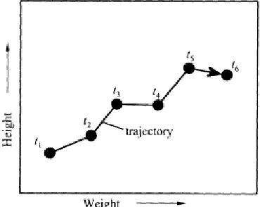
Standard phase space (hereafter just called phase space) is the phase space defined above: an abstract space in which coordinates represent the variables needed to specify the state of a dynamical system at a particular time. On a graph, a plotted point neatly and compactly defines the system's condition for some measuring occasion, as indicated by the point's coordinates (values of the variables). For example, we might plot a baby's height against its weight. Any plotted point represents the state of the baby (a dynamical system!) at a particular time, in terms of height and weight (Fig. 3.2). The next plotted point is the same baby's height and weight at one time interval later, and so on. Thus, the succession of plotted points shows how the baby grew over time. That is, comparing successive points shows how height has changed relative to weight, over time, t.
Figure 3.2
Standard phase space graph of baby's height and weight progression. The first measuring occasion
A line connecting the plotted points in their chronological order shows temporal evolution more clearly on the graph. The complete line on the graph (i.e. the sequence of measured values or list of successive iterates
plotted on a phase space graph) describes a time path or trajectory. A trajectory that comes back upon itself to form a closed loop in phase space is called an orbit.(The two terms are often used synonymously.) Each plotted point along any trajectory has evolved directly from (or is partly a result of) the preceding point. As we plot each successive point in phase space, the plotted points migrate around. Orbits and trajectories therefore reflect the movement or evolution of the dynamical system, as with our baby's weights and heights. That is, an orbit or trajectory moves around in the phase space with time. The trajectory is a neat, concise geometric picture that describes part of the system's history. When drawn on a graph, a trajectory isn't necessarily smooth, like the arcs of comets or cannonballs; instead, it can zigzag all over the phase space, at least for discrete data.
The phase space plot is a world that shows the trajectory and its development. Depending on various factors, different trajectories can evolve for the same system. The phase space plot and such a family of trajectories together are a phase space portrait, phase portrait,or phase diagram.
The phase space for any given system isn't limitless. On the contrary, it has rigid boundaries. The minimum and maximum possible values of each variable define the boundaries. We might not know what those values are.
A phase space with plotted trajectories ideally shows the complete set of all possible states that a dynamical system can ever be in. Usually, such a full portrayal is possible only with hypothetical data; a phase space graph of real-world data usually doesn't cover all of the system's possible states. For one thing, our measuring device might not have been able to measure the entire range of possible values, for each variable. For another, some combinations of values might not have occurred during the study. In addition, some relevant variables might not be on the graph, either because we don't know they are relevant or we've already committed the three axes.
Figure 3.3
For any system, there are often several ways to define a standard phase space and its variables. In setting up a phase space, one major goal is to describe the system by using the fewest possible number of variables. That simplifies the analysis and makes the system easier to understand. (And besides, if we want to draw a graph we're limited to three variables.) A pendulum (Fig. 3.3) is a good example. Its velocity changes with its position or displacement along its arc. We could describe any such position in terms of two variables—the x,y
coordinates. Similarly, we could describe the velocity at any time in terms of a horizontal component and a vertical component. That's four variables needed to describe the state of the system at any time. However, the two velocity components could be combined into one variable, the angular velocity. That simplifies our analysis by reducing the four variables to three. Furthermore, the two position variables x and y could be combined into one variable, the angular position. That reduces the number of variables to two—a situation much more
preferable than four.
Phase space graphs might contain hundreds or even thousands of chronologically plotted points. Such a graph is a global picture of many or all of the system's possible states. It can also reveal whether the system likes to spend more time in certain areas (certain combinations of values of the variables).
The trajectory in Figure 3.2 (the baby's growth) is a simple one. Phase space plots in nonlinear dynamics and chaos produce a wide variety of patterns—some simple and regular (e.g. arcs, loops and doughnuts), others with an unbelievable mixture of complexity and beauty.
Pseudo (Lagged) Phase Space
Maps
One of the most common terms in the chaos literature is map. Mathematically, a map (defined more completely below) is a function.And what's a function? As applied to a variable, a function is a "dependent" or output variable whose value is uniquely determined by one or more input ("independent") variables. Examples are the variable or function y in the relations y=3x, y=5x3-2x,and y=4x2+3.7z-2.66. In a more general sense, a function is
an equation or relation between two groups, A and B, such that at least one member of group A is matched with one member of group B (a "single-valued" function) or is matched with two or more members of group B (a "multi-valued" function). An example of a single-valued function is y=5x;for any value of x, there is only one value of y, and vice versa. An example of a multi-valued function is y=x2;for y=4, x can be +2 or -2, that is, one
value of y is matched with two values of x. "Function'' often means "single-valued function."
It's customary to indicate a function with parentheses. For instance, to say that "x is a function f of time t," people write x=f(t). From the context, it is up to us to see that they aren't using parentheses here to mean multiplication.
In chaos, a map or function is an equation or rule that specifies how a dynamical system evolves forward in time. It turns one number into another by specifying how x, usually (but not always) via a discrete step, goes to a new x. An example is xt+1=1.9-xt2 (Eq. 1.1). Equation 1.1 says that xt evolves one step forward in time (acquires
a new value, xt+1,) by an amount equal to 1.9-xt2 In general, given an initial or beginning value x0 (pronounced "x
naught") and the value of any constants, the map gives x1; given x1, the map gives x2; and so on. Like a
geographic map, it clearly shows a route and accurately tells us how to get to our next point. Figuratively, it is an input-output machine. The machine knows the equation, rule, or correspondence, so we put in x0 and get out
As you've probably noticed, computing a map follows an orderly, systematic series of steps. Any such orderly series of steps goes by the general name of an algorithm.An algorithm is any recipe for solving a problem, usually with the aid of a computer. The "recipe" might be a general plan, step-by-step procedure, list of rules, set of instructions, systematic program, or set of mathematical equations. An algorithm can have many forms, such as a loosely phrased group of text statements, a picture called a flowchart, or a rigorously specified computer program.
Because a map in chaos theory is often an equation meant to be iterated, many authors use "map" and
"equation" interchangeably. Further, they like to show the iterations on a graph. In such cases, they might call the graph a "map." "Map" (or its equivalent, "mapping") can pertain to either form—equation or graph.
A one-dimensional map is a map that deals with just one physical feature, such as temperature. It's a rule (such
as an iterated equation) relating that feature's value at one time to its value at another time. Graphs of such data are common. By convention, the input or older value goes on the horizontal axis, and the output value or function goes on the vertical axis. That general plotting format leaves room to label the axes in various ways. Four common labeling schemes for the ordinate and abscissa, respectively, are:
• "output x" and "input x"
• "xt+1, "and "xt"
• "next x" and "x"
• "x" and "previous x."
(Calling the graph "one-dimensional" is perhaps unfortunate and confusing, because it has two axes or
coordinates. A few authors, for that reason, call it "two dimensional." It's hard to reverse the tide now, though.)
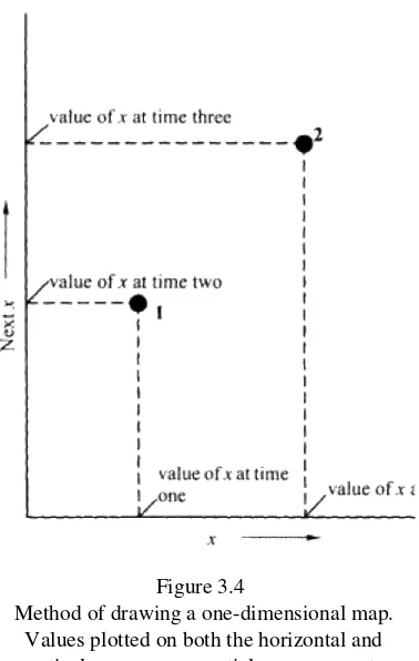
Plotting a one-dimensional map is easy (Fig. 3.4). The first point has an abscissa value of the input x ("xt") and
an ordinate value of the output x ("xt+1"). We therefore go along the horizontal axis to the first value of x, then
vertically to the second value of x, and plot a point. For the second point, everything moves up by one. That means the abscissa's new value becomes observation number two (which is the old xt+1), and the ordinate's new
value is observation number three, and so on. (Hence, each measurement participates twice—first as the ordinate value for one plotted point, then as the abscissa value for the next point.)
Each axis on a standard phase space graph represents a different variable (e.g. Fig. 3.2). In contrast, our graph of the one-dimensional map plots two successive measurements (xt+1 versus xt)of one measured feature, x.
Because xt and xt+1 each have a separate axis on the graph, chaologists (those who study chaos) think of xt and
xt+1 as separate variables ("time-shifted variables") and their associated plot as a type of phase space. However,
Figure 3.4
Method of drawing a one-dimensional map. Values plotted on both the horizontal and vertical axes are sequential measurements
of the same physical feature (x).
In the most common type of pseudo phase space, the different temporal measurements of the variable are taken at a constant time interval. In other cases, the time interval isn't necessarily constant. Examples of pseudo phase space plots representing such varying time intervals are most of the so-called return maps and next-amplitude maps,discussed in later chapters. The rest of this chapter deals only with a constant time interval.
Our discussion of sequential values so far has involved only two axes on the graph (two sequential values). In the same way, we can draw a graph of three successive values (xt, xt+1, xt+2). Analytically, in fact, we can consider
any number of sequential values. (Instead of starting with one value and going forward in time for the next values, some chaologists prefer to start with the latest measurement and work back in time. Labels for the successive measurements then are xt, xt+1, xt+2,and so on.)
Lag
Pseudo phase space is a graphical arena or setting for comparing a time series to later measurements within the same data (a subseries). For instance, a plot of xt+1 versus xt shows how each observation (xt) compares to the
next one (xt+1). In that comparison, we call the group of xtvalues the basic series and the group of xt+1 values the
subseries. By extending that idea, we can also compare each observation to the one made two measurements later (xt+2versus xt), three measurements later (xt+3 versus xt), and so on. The displacement or amount of offset, in
units of number of events, is called the lag.Lag is a selected, constant interval in time (or in number of
iterations) between the basic time series and any subseries we're comparing to it. It specifies the rule or basis for defining the subseries. For instance, the subseries xt+1 is based on a lag of one, xt+2 is based on a lag of two, and so
on.
A table clarifies lagged data. Let's take a simplified example involving xt, xt+1 and xt+2. Say the air temperature
outside your window at noon on six straight days is 5, 17, 23, 13, 7, and 10 degrees Centigrade, respectively. The first column of Table 3.1 lists the day or time, t. The second column is the basic time series, xt (the value of
x, here temperature, at the associated t). The third column lists, for each xt the next x (that is, xt+1). Column four
The columns for xt+1 and xt+2 each define a different subset of the original time series of column two. Specifically,
the column for xt+1 is one observation removed from the basic data, xt.That is, the series xt+1 represents a lag of
one (a "lag-one series"). The column for xt+2 is offset from the basic data by two observations (a lag of two, or a
"lag-two series"). The same idea lets us make up subsets based on a lag of three, four, and so on.
Table 3.1 Hypothetical time series of six successive noon temperatures and lagged values.
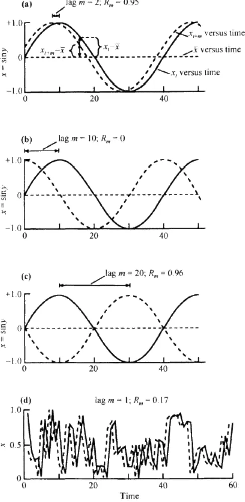
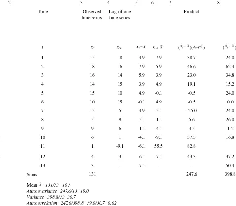
One way to compare the various series is statistically. That is, we might compute certain statistics for each series. Table 3.1, for example, shows the average value of each series. Or, we might compute the
autocorrelation coefficient (Ch. 7) for each series. The statistical approach compares the two series on a group basis. Another way to compare the two series is graphically (e.g. Fig. 3.4). In the following paragraphs, we'll deal with the graphical comparison. Both approaches play a key role in many chaos analyses.
Two simple principles in defining and plotting lagged data are:
• The first axis or coordinate usually (but not always) is the original time series, xt. Unless we decide
otherwise, that original or basic series advances by one increment or measurement, irrespective of the lag we choose. That is, each successive value in the xtseries usually is the next actual observation in the time
series (e.g. Table 3.1, col. 2).
• The only role of lag is to define the values that make up the subseries. Thus, for any value of xt the
associated values plotted on the second and third axes are offset from the abscissa value by the selected lag. Lag doesn't apply to values in the xt series.
To analyze the data of Table 3.1 using a lag of two, we consider the first event with the third, the second with the fourth, and so on. ("Consider" here implies using the two events together in some mathematical or graphical way.) On a pseudo phase space plot, the abscissa represents xt and the ordinate xt+2. The value of the lag (here
two) tells us how to get the y coordinate of each plotted point. Thus, for the noon temperatures, the first plotted point has an abscissa value of 5 (the first value in our measured series) and an ordinate value of 23 (the third value in the basic data, i.e. the second value after 5, since our specified lag is two). For the second plotted point, the abscissa value is 17 (the second value in the time series); the ordinate value is two observations later, or 13 (the fourth value of the original series). The third point consists of values three and five. Thus, xt is 23 (the third
measurement), and xt+2 is 7 (the fifth value). And so on. The overall plot shows how values two observations
apart relate to each other.
The graphical space on the pseudo phase space plot of the data of Table 3.1 is a lagged phase space or, more simply, a lag space. Lagged phase space is a special type of pseudo phase space in which the coordinates represent lagged values of one physical feature. Such a graph is long-established and common in time-series analysis. In chaos theory as well, it's a basic, important and standard tool.
Some authors like to label the first observation as corresponding to "time zero" rather than time one. They do so because that first value is the starting or original value in the list of measurements. The next value from that origin (our observation number two in Table 3.1) then becomes the value at time one, and so on. Both numbering schemes are common.
Embedding dimension
A pseudo (lagged) phase space graph such as Figure 3.4 can have two or three axes or dimensions. Furthermore, as mentioned earlier in the chapter, chaologists often extend the idea of phase space to more than three
dimensions. In fact, we can analyze mathematically—and compare—any number of subseries of the basic data. Each such subseries is a dimension, just as if we restricted ourselves to three of them and plotted them on a graph. Plotting lagged values of one feature in that manner is a way of"putting the basic data to bed" (or
embedding them) in the designated number of phase space axes or dimensions. Even when we're analyzing
them by crunching numbers rather than by plotting, the total number of such dimensions (subseries) that we analyze or plot is called the embedding dimension,an important term. The embedding dimension is the total number of separate time series (including the original series, plus the shorter series obtained by lagging that series) included in any one analysis.
The "analysis" needn't involve every possible subseries. For example, we might set the lag at one and compare
xt with xt+1,(an embedding dimension of two). The next step might be to add another subgroup (xt+2) and consider
groups xt, xt+1 and xt+2 together. That's an embedding dimension of three. Comparing groups xt, xt+1, xt+2, and xt+3
means an embedding dimension of four, and so on.
From a graphical point of view, the embedding dimension is the number of axes on a pseudo phase space graph. Analytically, it's the number of variables (xt, xt+1,etc.) in an analysis. In prediction, we might use a succession of
lagged values to predict the next value in the lagged series. In other words, from a prediction point of view, the embedding dimension is the number of successive points (possibly lagged points) that we use to predict each next value in the series.