ORIGINAL ARTICLE
Reentrant FMS scheduling in loop layout with consideration
of multi loading-unloading stations and shortcuts
Achmad P. Rifai1&Siti Zawiah Md Dawal1&Aliq Zuhdi1&
Hideki Aoyama2&K. Case3
Received: 31 August 2014 / Accepted: 5 June 2015
#Springer-Verlag London 2015
Abstract The scheduling problem in flexible manufacturing systems (FMS) environment with loop layout configuration has been shown to be a NP-hard problem. Moreover, the im-provement and modification of the loop layout add to the difficulties in the production planning stage. The introduction of multi loading-unloading points and turntable shortcut re-sulted on more possible routes, thus increasing the complex-ity. This research addressed the reentrant FMS scheduling problem where jobs are allowed to reenter the system and revisit particular machines. The problem is to determine the optimal sequence of the jobs as well as the routing options. A modified genetic algorithm (GA) was proposed to generate the feasible solutions. The crowding distance-based substitu-tion was incorporated to maintain the diversity of the popula-tion. A set of test was applied to compare the performance of the proposed approach with other methods. Further computa-tional experiments were conducted to assess the significance of multi loading-unloading and shortcuts in reducing the makespan, mean flow time, and tardiness. The results highlighted that the proposed model was robust and effective in the scheduling problem for both small and large size problems.
Keyword Reentrant FMS scheduling . Multi loading-unloading and shortcuts . Genetic algorithm . Crowding distance-based substitution
1 Introduction
FMS are important systems to satisfy the flexibility and pro-ductivity needs of manufacturing enterprises. A FMS typically consists of CNC machines with automated tool magazines, material handling systems, and computer workstations, con-nected together mechanically and controlled by a computer control system. Operation management in FMS is an intracta-ble task for engineers as well as technical manager due to the complexity of the systems. Therefore, to manage the FMS effectively, more performance-related decision-making is im-plemented when compared to conventional manufacturing systems, which use a transfer line or job shop production system [1].
FMS covers a wide variety of automated manufacturing systems. A loop layout, consisting of several machines con-nected by a material handling system in circular form, is one of the most commonly used configurations in FMS. Material flows and part routes in FMS using loop layouts are more complex than the in-line layout. Due to its cyclical nature, the machine visiting sequence of a part is different from its operation sequence, depending on the machine arrangement. Previous studies have concerned about the improvement in loop layout configurations. Recently, the addition of multi loading-unloading (L/U) stations and shortcuts greatly im-proves the performance of loop layout configurations with significant decreases in the traveling distance [2,3]. However, the improvements increase the complexity of the loop layout system. As a result, improvements in production planning and control are also required. Scheduling, considered as the heart * Achmad P. Rifai
Siti Zawiah Md Dawal [email protected]
1
Department of Mechanical Engineering, Faculty of Engineering, University of Malaya, 50603 Kuala Lumpur, Malaysia
2
School of Integrated Design Engineering, Keio University, Tokyo, Japan
3 Mechanical and Manufacturing Engineering, Loughborough
of production planning and control, is also affected and needs to be updated.
The scheduling problem of FMS is known to be a NP-hard problem where the increase of problem size causes the times to solve the optimization problem to escalate exponentially. Moreover, production planning and control in FMS are more difficult than those of mass production systems [4]. FMS can process different parts while using the same configuration of machines where each machine in FMS can perform various operations. The combinatorial characteristic of the assign-ments and tasks sequencing decisions encountered is the source of complexity of scheduling in FMS. In addition, FMS scheduling also takes into account the technological, capacity, and availability constraints as the limiting resources, such as machines, buffers, tools, and material handling de-vices [5].
Studies on the scheduling aspect are required to catch up with the improvement in the design sector. Since most previ-ous research addressed the scheduling problem for simple loop layout based FMS, improved scheduling models are needed to accommodate the addition and modification in loop layout based FMS. The improvements in layout design in-crease the complexity of the scheduling problems. Hence, improvement in the optimization method is essential to solve the scheduling problem effectively and efficiently. This re-search deals with the reentrant FMS scheduling problem with consideration of the improvements in the loop layout design. In particular, the scheduling model for accommodating the issues in addition of multi L/U stations and turntable shortcut in loop layout configurations is considered as the main contri-bution. A modified GA is proposed to determine near optimal solutions within acceptable solution times. The approach em-ploys a substitution based on crowding distance to replace the individuals with close proximity. The use of meta-heuristic techniques is necessary since the FMS scheduling problem is more complicated than scheduling in a conventional system. Furthermore, discrete event simulation based modeling is de-veloped to verify the outcome of the model. The simulation is used to validate and evaluate the part schedule and routing options generated by the modified GA approach.
The rest of the article is organized as follows. Section2 provides a brief literature review of FMS scheduling. Section3 presents the definition and formulation of the scheduling prob-lem in loop layout based FMS. Section4 explains the pro-posed approach. In Sect.5, numerical results and simulation experiments are reported and discussed. Finally, conclusions are outlined in Sect.6.
2 Literature review
FMS scheduling has been an active research area because of its importance in the today’s manufacturing industry. Due to a
high degree of product variability in FMS, the part routing and part flows are of considerable concern. There are two opera-tional policy in the FMS scheduling. The first is the tool movement policy where parts are assigned to machines and necessary tools are brought to the machines to finish the op-erations. The second option is part movement policy where parts are transferred from one machine to the others based on the operation process. Part movement policy is implemented in most manufacturing systems because it has the advantage of ensuring that all parts can be processed using the capabili-ties of the machines. Besides that, there has been research of other scheduling problems such as that by Hall et al. [4] which considered the material handling scheduling. Some studies have also attempted to integrate part scheduling with tool se-lection and/or material handling scheduling like the study by Gamila and Motavalli [5] and Zeballos et al. [6]. Nevertheless, the majority of the research considered the part movement policy as the main concern.
unloading points with one AGV to transport the parts be-tween machines.
The previous studies did not necessarily highlight the same problems as they differed in the type of FMS, scheduling problems, scheduling type and the objective functions used. Joseph and Sridharan [17] evaluated the effect of dynamic due-date assignment models, routing flexibility levels, se-quencing flexibility levels and part sese-quencing rules on the performance of FMS in standard loop configurations. The study proposed the development of a model called dynamical-ly estimated flow allowance (DEFA). Cardin et al. [18] pre-sented the group scheduling method using an emulation of a complex FMS with loop configuration. The study focused on determining the ability of the group scheduling in absorbing uncertainties in complex FMS. Udhayakumar and Kumanan [19] addressed the integration between production schedule and material handling schedule for a U Loop layout in the FMS. In the first phase, the FMS production schedule, with minimizing makespan as the objective function, was generat-ed using the Giffler and Thompson algorithm. Then, the out-put of production scheduling was used to develop material handling schedules.
Hsu et al. [20] attempted to minimize the work in process to satisfy economic constraints. A two-step resolution approach was presented to solve the problem. Petri net modelling of the production process was applied for constructing the model of the problem. Afterward, a genetic algorithm was used to ob-tain the sequence of tasks for a flexible manufacturing cell. In addition to the static environment, dynamic scheduling has been developed as an alternative approach to mimic real-life dynamic environments. Qin et al. [21] examined dynamic scheduling for an interbay automated material handling sys-tem configuration. The configuration was a single loop, spine type interbay material handling route. The AGVs moved around the path in unidirectional movement. Alternative shortcut paths were placed to connect the upper and lower rows of the main loop. A genetic programming based CDR generator was proposed to generate the composing dispatching rule that can be used in real-life dynamic produc-tion. The dispatching of AGV in the FMS was also concerned by Caridá et al. [22] in which the factory layout was modeled in Petri nets.
Objective functions hold the central role for optimization in FMS scheduling problems. Several measurements have been used as the indicators of system performance. Minimizing makespan is the most common objective function, as indicat-ed by researchers in the FMS schindicat-eduling problems [23–27].
Other research has tried to use other approaches, i.e. reducing work in process [20,28]. However, in practical applications, there are many objectives that have been considered in sched-uling problems. This has indicated that evaluating a single objective is not satisfactory for improving the performance of the complete manufacturing systems [29]. In addition,
satisfying a single objective cannot resolve the trade-off be-tween criteria. Therefore, it is important to consider multiple objective functions simultaneously since a greater variety of performance indicators can be accommodated. Joseph and Sridharan [17] employed mean flow time, mean tardiness, percentage of tardy parts and mean flow allowance. Prakash et al. [30] utilized bi-objective functions which are mean flow time and throughput to quantify performance. Jerald et al. [12] aimed to minimize idle time and the penalty cost for not meet-ing delivery dates by proposmeet-ing simultaneous schedulmeet-ing of parts and AGV. Ebrahimi et al. [31] used the combination of minimizing makespan and tardiness. These criteria represent the two important issues in the industries, the maximizing productivity of line production and fulfilling the customer expectation.
Related to the methods used, there are two categories of approach: optimization methods for exact solutions using mathematical programming and meta-heuristic algorithms for near optimal solutions. An example of the use of mathe-matical programming methods is the branch and bound solu-tion method proposed by Das and Canel [10] to exploit the special structure of the problem in developing strong lower bounds. The problem was modeled for a MCFMS with flowshop characteristics. A MCFMS consists of a number of flexible manufacturing cells, and possibly a number of single flexible machines, connected by an automated material han-dling system. Minimizing makespan was set as the objective function.
In recent research, meta-heuristic became the trend of re-lated studies since they possess the learning ability, which the traditional scheduling techniques do not have [32]. Some meta-heuristics have been shown to provide good perfor-mance solutions in previous studies. Low et al. [33] proposed the combination of Simulated Annealing (SA) and Tabu Search (TS). The hybrid heuristic was used to solve the ad-dressed FMS scheduling problem with three performance in-dicators, mean flow time, mean machine idle time, and mean job tardiness, simultaneously. Two heuristic procedures from their previous work [34] called sequence-improving proce-dure (SIP) and routing-exchange proceproce-dure (REP) were im-plemented using SA and TS. As a result four different hybrid searching structures were generated, depending on which searching procedure was adopted in REP and SIP, respective-ly. Baruwa and Piera presented timed colored Petri nets, com-bining evaluation methods (simulation) and search methods (optimization) [35]. The proposed approach was aimed to find the near optimal solutions in short computation time. Other methods commonly used in the scheduling problems belong to Swarm intelligence family, including ant colony optimiza-tion [36], pheromone approach [37] and chemotaxis-enhanced bacterial foraging algorithm [38].
[39] developed a network-based hybrid GA. The proposed method was combined with the neighborhood search tech-nique in a mutation operation to improve the solution of the FMS problem and to enhance the performance of the genetic search process. Prakash et al. [30] developed a novel approach called a knowledge based genetic algorithm (KBGA) by com-bining GA with knowledge management. Godinho Filho et al. [40] reviewed the use of genetic algorithms to solve schedul-ing problems in FMS. There were four conclusions from this literature study: (i) there was a switch of direction where meta-heuristics, especially GA and its hybrid have become popular (ii) although most studies dealt with complex environments concerning both the routing flexibility and the job complexity, only a minority of papers simultaneously considered the vari-ety of possible capacity constraints on an FMS environment (iii) local optimization methods were rarely used; (iv) makespan was the most widely used measurement of perfor-mance. In summary, the GA has proven successful when im-plemented in various FMS scheduling problems. Thus, it is worth developing a modified GA for further study.
From the point of view of layout system complexity, pre-vious studies considered relatively simple configuration. Meanwhile, the loop layout configuration has recently been extensively modified to increase its performance and flexibil-ity. Some examples of improvement in the loop layout design are the addition of turntable shortcuts [2] and multi loading-unloading points [3]. Since these additions have not previous-ly been included, more studies are required to cover the gap in the complex loop layout system. Thus, based on the literature review and our best knowledge, this study emphasizes the development of a part scheduling model for complex loop layout in FMS. The model accommodates the addition of multi loading-unloading points and turntable shortcut in the configuration. A modified GA with crowding distance based substitution is proposed to solve the reentrant FMS scheduling problem.
3 Problem formulation
3.1 Reentrant FMS scheduling
Loop layout consists of several machines connected by mate-rial handling in a circular form. The reentrant characteristic allows the part to reenter the system and revisit particular parts, thus forming cyclic traveling routes. In this study, the term of job and part are interchangeable, in which both indi-cate the same meaning. Scheduling in FMS can be considered as the combination of flowshop and jobshop scheduling with additional constraints. Figure1illustrates the example config-uration of the modified loop layout.
An example taken from previous literature [19] with addi-tional properties is presented to illustrate the scheduling
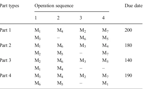
problem in loop layout FMS. There are four parts to be proc-essed in seven different machines with distinct due dates. In particular operations, there are alternative machines which can be used to substitute the main machine. Thus, there are many possible routing options for the parts. The number of possible processing sequence depends on the alternative machines, which can be calculated as 2n, wherenis the number of alter-native machines corresponding to each part. Table1shows an example of operation sequence.
In the example, the number of alternative machines n=3 that can be used to process part 1, thus there are 23=8 possible processing sequence. The parts are allowed to enter and exit from the system which results in minimum travel distance. The parts enter using the nearest loading point prior to the machine used to process the first operation, and exit from the nearest unloading point subsequent to the machine used to process the last operation. The model is also built based on the assumption that whenever circumstances are possible, a shortcut is always used to minimize the travel distance.
This study addresses the determination of two criteria in production planning, the part dispatching schedule and routing choice. The dispatching schedule is a permutation variable that indicates the dispatching sequence of the parts. Since this study covers the multi loading and unloading point addition, the permutation characteristic is exclusively applied
Buffer 7
Fig. 1 Example of modified loop layout configuration
Table 1 Example of operation sequence matrix
Part types Operation sequence Due date
for the parts at the same loading point. Unlike in conventional manufacturing systems, FMS allows the parts to be processed by alternative machines for particular operations. This condi-tion results in the various routing opcondi-tions for the parts. The routing choice not only determines the machine visiting se-quence, but also the processing time and setup time for each operation that will affect the completion time of the parts. Thus, the proposed model considers the routing choice of each part to get the most optimized schedule.
3.2 Mathematical model
The FMS considered consists of a set of machinesJ, which are arranged in a cyclic layout connected with a conveyor. There are several shortcuts inside in particular positions. The main conveyor of the loop is unidirectional, while the shortcuts’
conveyor is bidirectional. Beside the main loading-unloading point, there are extra loading-unloading points placed inside the loop. These points can either contain only loading or unloading points or can also contain both loading-unloading points. The parts can enter the system using any loading pointl and leave the system as a product from any unloading pointu. There is a set of partsKthat must be processed. A set of operationsIcorresponding to partkis processed by specific machinej. Every process follows the job sequence of each part denoted bySk. This means that an operationiktof partkcannot
be processed before the predecessor operationikt−1has been completed. The transport time is denoted byτ, which depends on distance to be traveled by the part to perform operationi after completion of operationi−1, denoted byd. In the case of
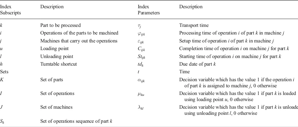
transport time in shortcuts and from/to loading-unloading points, the same symbol is applied. Table2lists the notations use in the mathematical model.
The machines can only process one part at the same time. The parts will be placed in the buffer which is positioned just before the machine if there is another part being processed by that machine. The duration between the parts entering the buffer until the part enters the machine is described as delay d. The manufacturing process of partkin machinejwill take some time expressed by the processing timeφijk. In FMS, each
machine can perform various operations for different parts. However, a particular time is needed to setup the machine before processing a different type of parts. This is denoted by the setup timeεijkwhich corresponds to partkand machine j.1.
Multi-objective functions, consisting of minimizing makespan Cmax, mean flow timeTf and tardinessTt, were used as the approach to measuring production efficiency and resource utilization. The objective functions also represent the interest in the real problem faced by the manufacturing indus-tries [20].
Equations 1,2, and 3 describe the objective functions, which are makespan, mean flow time, and total tardiness, respectively. Cijkis the integer value of the completion time
of operationion machinejfor each partk. tdkis the due date of
partk. The total fitness is the sum of each objective function
Table 2 Lists of notations
Index Description Index Description
Subscripts Parameters
k Part to be processed τj Transport time
i Operations of the parts to be machined φijk Processing time of operationiof partkin machinej
j Machines that carry out the operations εijk Setup time of operationiof partkin machinej
u Loading point Cijk Completion time of operationion machinejfor partk
l Unloading point Stijk Starting time of operationion machinejfor partk
h Turntable shortcut tdk Due date of partk
Sets t Time
K Set of parts αijk Decision variable which has the value 1 if the operationi
of partkis assigned to machinej, 0 otherwise
I Set of operations μku Decision variable which has the value 1 if partkis loaded
using loading pointu, 0 otherwise
J Set of machines λkl Decision variable which has the value 1 if partkis unloaded
using unloading pointl, 0 otherwise
with equal weighting factor. Thus, each objective function has equal significance. The objective functions are subject to the following constraint.
Equation4 states that one machine must be selected for each operation.αijkis a decision variable which will have
the value 1 if theith operation of partkis assigned to machine j, and 0 otherwise. Equation5 ensures that the completion time of operationion machine jfor partk, must be greater than the predecessor operationi−1, by at least the processing
time required for an operationiplus transport time and setup time for operationiof partkon machinej. Equation6defines the transport time which is calculated by the distance between machinejused to process operationiand machinej’used to process operationi’.
Equation7 defines that each operation begins after time zero. Equation8describes the nonzero property of completion time operationiof partk. Equations9and10ensure that the parts can only be loaded and unloaded by one loading and one unloading station. Note thatμku=1 if partkis loaded by
load-ingu. Similarly,λkl=1 if partkis unloaded using unloadingl,
0 otherwise. Equation 11ensures that the starting time of operationiof partkmust not be earlier than the sum of com-pletion time of the predecessor operationi−1 of the same job and the transport time.
4 Proposed approach
In solving the scheduling and assignment problems of FMS, past studies have adopted mathematical program-ming techniques. However, in real-world problem in-stances, it has been seen that the traditional techniques
cannot reach optimal solutions [17]. Thus, the use of meta-heuristic optimization, also known as artificial intel-ligence techniques, has been considered. This study ad-dresses the use of a modified genetic algorithm to solve the scheduling problem. The GA aims to seek the optimum value of objective functionfwhich is influenced by a vec-tor of decision variables x. Each individual represents a potential solution to the problem at hand. Then, the indi-vidual is evaluated to give some measures of its fitness. Some individuals experience stochastic transformation by means of genetic operations to form new individuals. There are two types of transformation: crossover, which creates new individuals by combining parts from two par-ent individuals, and mutation, creating new individuals by making changes in a single chromosome.
One of the keys to good performance in GAs is main-taining the diversity where it should be prominent in any application [41]. In the GA, the nature of crossover leads to premature convergence since it tends to produce uniform offspring. Moreover, the implementation of roulette wheel selection allows the good individuals to be selected repeat-edly. This condition results in difficulty in maintaining the population diversity. As a solution, the modified GA incor-porates the crowding distance to evaluate the similarity between individuals. Individuals’substitution engaging
the elitist based re-combination and re-mutation method is used to produce the substitute. The scheme of the proposed approach is illustrated in Fig.2.
After several generations, the algorithm converges to the best individual, which represents an optimal solution. The GA parameters in the proposed approach are set as follows: the population sizePs=20, crossover ratePc=0.8, and mutation ratePm=0.025 [12,42]. The loop process continues until the termination criterion is fulfilled, when the numbers of gener-ationsN=100.
4.1 Coding representation
The GA process starts with coding representation. In optimi-zation problems of FMS scheduling, the main decision vari-able is the sequence of each part that will enter the system. Each part number may be considered to be a gene on chromo-some represented using integer permutation chromochromo-somes. Since each gene represents a part number, the greater number of parts means longer chromosomes. Table3depicts the inte-ger permutation chromosomes; the numbers represent the part codes.
depending on the operations, layout structure, and the alterna-tive machines that can be used to process the part.
4.2 Parent selection
The initial population of solutions is produced by utilizing a stochastic technique. A set of decision variables is portrayed by coded strings of finite length. A roulette wheel is employed as the parent selection method, in which the probability of an individualibeing selected is dependent on its fitness valuefi as defined in Eq.12.
pi¼f i.X n¼1
i¼1
f i ð12Þ
When the inequalityp0+p1+…+pi−1<γ≤p0+p1+…+
pi−1+piis met, the individualiis selected for the next
gen-eration. To ensure that good chromosomes have a higher pos-sibility of being picked, ranking schemes are always adopted. This scheme is performed by sorting the population on the basis of fitness values and then the selection operation is un-dergone based upon the rank. Therefore, individuals with high fitness values have a greater chance of being chosen as parents.
4.3 Crossover
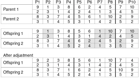
The crossover operator used in this research is a partially matched crossover (PMX). The crossover operator divides each selected individual into two or more sections and swaps the divided sections of the individual. Figure3illustrates the crossover operation involving PMX techniques.
4.4 Mutation
Since an integer permutation representation is used in this study, the exchange mutation, also called swap mutation, is applied. In this technique, two genes are picked randomly and their alleles get exchanged. Figure4shows the mutation pro-cess using swap mutation.
Unlike the crossover which operates on the individual level (swapping certain parts between two individuals), mutation operators operates on the gen level. Therefore, the process may result to an infeasible string where route choices may not be available. To accommodate this issue, we perform an adjustment process for allele value which violates the con-straints, i.e., the value of selected route exceeds the number of possible routes. The new values are randomly generated among all possible routes.
4.5 Crowding distance calculation
The level of population diversity can be estimated using crowding distance, which is an estimate of the perimeter of the cuboid formed by using the nearest neighbors as the ver-tices [43]. The proposed approach uses the genotype based crowding distance, calculated using the Euclidean distance. Since there are two variables to be optimized, the computation uses a two dimension average Euclidean distance calculation, Start Fig. 2 Scheme of modified GA
Table 3 Integer permutation chromosome illustration
P1 P2 P3 P4 P5 P6 P7 P8 P9 P10
presented in Eq.13.
wherep is the allele value of individualiandqis the allele value of individuali−1. Subscriptxrepresents the part
sched-ule. Subscriptyrepresents the routing options. The order of allele is represented byn, where Nindicates the length of chromosomes. The distance computation requires sorting the population according to objective function value in descend-ing order of magnitude. In this scheme, the elitist individual will always be kept. Individuals which have close proximity with the predecessor solutions will be replaced.
4.6 Individuals substitution
The distance computation results in several solutions which do not meet the threshold. To maintain the fixed population size, new generated offspring are used as substitutes from the replaced individuals. The substitution of an individual in-volves two genetic processes, re-combination and re-muta-tion, to generate distinct solutions. Re-combination is based on the crossover approach involving the elitist individual and the individual to be replaced. Re-mutation is achieved by changing an allele with a new randomly generated value.
4.7 Population replacement
Having finished the genetic operator, elitism is applied to allow the best solution to be preserved in the next genera-tion. In this scheme, the surviving best solution replaces the worst individual, which either comes from the previous iteration or as the result of the crossover and mutation op-erators. Thus, the good offspring will not be lost due to population replacement.
5 Results and discussion
5.1 Datasets and layout properties
The proposed approach was tested to measure perfor-mance. The test beds were taken from previous literatures [44–46,19] with some modifications to conform the FMS
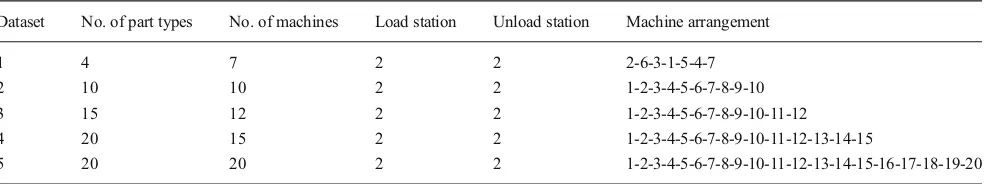
environment. The jobs visit the machines in an operation sequence with the choice of selecting alternative machines for the operations. The operation sequence for each job is a random permutation of the machines, while the processing times and setup times are uniformly distributed. Each job has a deadline, which is uniformly distributed on an inter-val determined by the expected workload of the system and other parameters. Since the datasets lack some of the pa-rameters, such as setup time and deadline, the missing data were generated artificially. The layout properties were af-fected by the datasets used, especially the number of ma-chines, parts and operation sequence. The details of point to point distance between machines and layout properties are given in Appendixes 1 and 2, respectively. Table 4 shows the instances used to test the algorithms.
5.2 Improvement and robustness test
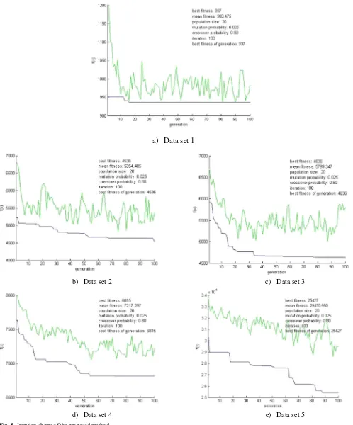
A comparative study was conducted to measure the perfor-mance of the proposed genetic algorithm optimization model. The approach was contrasted with dispatching rule techniques such as shortest processing time (SPT), longest processing time (LPT), earlier due date (EDD), and other meta-heuristics, such as conventional GA and SA. The comparison was based on the objective functions which are minimizing makespan, mean flow time, and total tardi-ness. The experiments were done by ten repetitions for each method. Figure 5presents the iteration charts of the modified GA in each dataset. The upper line represents the average fitness of the generation. The lower line represents the best fitness obtained.
The iteration process indicated that in small datasets, e.g., dataset 1, the GA quickly reached a stable state because there was only a small solution space to be explored. Meanwhile, in large datasets, there were huge solution spaces with many
P1 P2 P3 P4 P5 P6 P7 P8 P9 P10
Fig. 4 Mutation process using swap mutation
Table 4 Data sets and configurations for the case studies
Dataset No. of part types No. of machines Load station Unload station Machine arrangement
1 4 7 2 2 2-6-3-1-5-4-7
2 10 10 2 2 1-2-3-4-5-6-7-8-9-10
3 15 12 2 2 1-2-3-4-5-6-7-8-9-10-11-12
4 20 15 2 2 1-2-3-4-5-6-7-8-9-10-11-12-13-14-15
combinations of sequences and possible routing options. Thus, the searching process in large datasets took more itera-tions to converge than in small datasets. Besides comparison
of each objective function, the total fitness was also contrasted. The improvement rateIRof the proposed approach over methodAis defined in Eq.14.
b) Data set 2 c) Data set 3
d) Data set 4 e) Data set 5
a) Data set 1
Table 5 Value of objective functions obtained and improvements
Indicator Method Datasets
1 2 3 4 5
Makespan SPT 330 1852 1358 945 4669
LPT 382 1880 1220 962 4465
EDD 382 1773 1357 1040 4624
SA 322 1769 1248 955 4294
GA 322 1768 1308 889 4525
Modified GA 322 1727 1219 900 4147
Mean flow time SPT 265 1616 1121 722 3873
LPT 302 1648 1058 731 3810
EDD 302 1591 1122 721 3883
SA 265 1557 1056 713 3719
GA 265 1547 1030 688 3635
Modified GA 265 1493 1023 684 3622
Total tardiness SPT 349 1923 3749 5662 22,750
LPT 499 2240 2803 5848 21,381
EDD 498 1703 3756 5655 22,843
SA 350 1440 2804 5489 19,972
GA 350 1328 2519 4980 18,363
Modified GA 350 997 2366 4910 17,658
Total fitness SPT 944 5391 6228 7329 31,292
LPT 1183 5768 5081 7541 29,656
EDD 1182 5067 6235 7416 31,350
SA 937 4766 5108 7157 27,985
GA 937 4643 4857 6557 26,523
Modified GA 937 4217 4608 6494 25,427
Improvement rateIRof modified GA over SPT 0.74 % 21.78 % 26.01 % 11.39 % 18.74 %
LPT 20.79 % 26.89 % 9.31 % 13.88 % 14.26 %
EDD 20.73 % 16.78 % 26.09 % 12.43 % 18.89 %
SA 0.00 % 11.52 % 9.79 % 9.26 % 9.14 %
GA 0.00 % 9.18 % 5.13 % 0.96 % 4.13 %
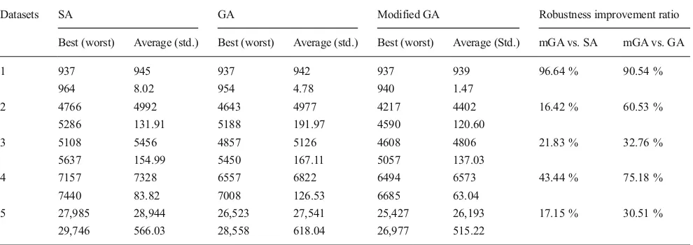
Table 6 Robustness improvement ratio of modified GA, in contrast to SA and GA
Datasets SA GA Modified GA Robustness improvement ratio
Best (worst) Average (std.) Best (worst) Average (std.) Best (worst) Average (Std.) mGA vs. SA mGA vs. GA
1 937 945 937 942 937 939 96.64 % 90.54 %
964 8.02 954 4.78 940 1.47
2 4766 4992 4643 4977 4217 4402 16.42 % 60.53 %
5286 131.91 5188 191.97 4590 120.60
3 5108 5456 4857 5126 4608 4806 21.83 % 32.76 %
5637 154.99 5450 167.11 5057 137.03
4 7157 7328 6557 6822 6494 6573 43.44 % 75.18 %
7440 83.82 7008 126.53 6685 63.04
5 27,985 28,944 26,523 27,541 25,427 26,193 17.15 % 30.51 %
I R¼ f i Að Þ−f i mGAð Þ
f i Að Þ 100% ð14Þ
wherefi(mGA) denotes the total fitness obtained by the pro-posed approach andfi(A) denotes the total fitness obtained by heuristics methodA. Table5 shows the best results of each method and the improvements, in term of total fitness, obtain-ed by the proposobtain-ed approach comparobtain-ed to other methods.
Based on the numerical results, the modified GA outperformed the other methods in all case studies in terms of
overall fitness value. The results of case studies also depicted the consistency of modified GA, either applied in small or large datasets. To further examine the performance of modified GA, this study calculates the robustness improvement ratio in con-trast to the simple GA and SA as defined in Eqs.15and16. The results of robustness test are described in Table6.
Robustness improvement ratio in contrast to simple GA
¼ 1−σ 2ðmGAÞ
σ2ðGAÞ 100% ð15Þ
Data set 1 Data set 4 With substitution
Data set 2 Data set 5 Without substitution
Data set 3
Robustness improvement ratio in contrast to SA
¼ 1−σ 2ðmGAÞ
σ2ðSAÞ 100% ð16Þ
The results demonstrated a significant robustness improve-ment of modified GA relative to simple GA and SA both in small and large data. The improvement was more prominent against the simple GA. GA tends to narrow its search space to small neighborhoods when it finds a local optima and failed to explore better solutions in other neighborhoods. When the ex-periments were replicated, the search space of simple GA was focused to different neighborhoods, thus it has the lowest stan-dard deviation. In contrast to simple GA, SA has better ability to explore wider neighborhoods. However, the fitness obtained by SA was lower than GA and modified GA. Although SA had better robustness than GA, it was less effective. In modified GA, the crowding distance based substitution gives more op-portunity to broaden the search space without discarding the current neighborhoods. Therefore, the modified GA was more stable, robust and effective than other methods.
5.3 Similarity level analysis
A similarity level analysis was carried out to measure the robustness of the proposed approach. The comparison used the crowding distance as an approach to determine the simi-larity level. Figure6presents the comparison of the crowding distance before and after the individual substitution in each
generation. The graphs indicate that the earlier generations had a low similarity level. Since the initial population was stochastically generated, the individuals have a high degree of diversity. As the iteration process continues, the diversity level decreases. The crossover and roulette wheel selection causes individuals to move toward convergence because rou-lette wheel selection allows the individuals with good fitness to be selected with high probability. As a result, the good individuals dominate the next iteration and increase the simi-larity level in that generation.
The increasing of similarity results in premature convergence since the algorithm will fail to explore new solution space. Due to this effect, the simple GA is prone to be caught in subopti-mum solutions. The results of experiments indicated that the simple GA failed to obtain better solutions as observed in the Table6. It was proved that the GA was trapped in premature convergence. As a solution, the proposed modified GA ap-proach was intended to solve the similarity level. The apap-proach involves pairwise comparison between individuals. When a pair of individuals has a low crowding distance, the worse solution will be substituted with a newly generated solution.
As indicated by Table 7, the individual substitutions in-creased the average distance and reduced the similarity level. It effectively improved the population diversity in all in-stances, thus reducing the possibility of being trapped in pre-mature convergence. The trend of the improvement rate shows that small problems have higher sensitivity to the substitution and the large data sets are more resistant toward the change. In the instance with fewer parts to be processed, the modification of a gene will significantly alter the overall fitness of the chro-mosomes. Thus, it can be stated that the number of parts affects the improvement rate on diversity.
5.4 Significance of multi L/U and shortcuts
The performance of FMS is affected by the jobs’ operation
routes as well as the traveling routes of the parts. In case of the configuration discussed, the addition of extra loading-unloading and shortcuts offer the alternative of part traveling
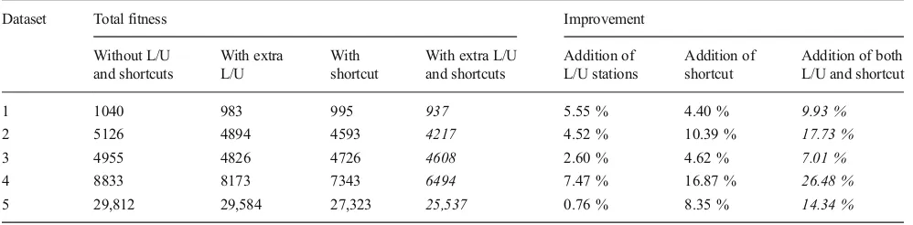
Table 8 Improvement obtained by adding extra L/U stations and shortcut
Dataset Total fitness Improvement
Without L/U
The highlighted values (lowest total fitness and highest improvement) have been pointed out in italics Table 7 Average Euclidian distance
Data set Euclidian distance Improvement
on diversity Without substitution With substitution
1 0.053 0.068 28.30 %
2 0.485 0.533 9.90 %
3 1.731 1.867 7.86 %
4 2.289 2.369 3.49 %
routes. This section presents the analysis of the significance of extra loading-unloading stations and shortcut addition into the loop layout in reducing the objective functions, makespanC -max, mean flow timeTf, and tardinessTt.
A set of computational experiments was carried out by examining the four types of configurations, which are the simple loop layout, the addition of extra loading-unloading station only, the addition of shortcut only and the addition of both extra loading-unloading stations and shortcut. The posi-tion of loading-unloading staposi-tions and shortcut were randomly generated among the feasible position with assumption the number of L/U stations l=1, u=1, and shortcut h=1. The
experiments were based on the same parameters to ensure the performance stability of the proposed approach.
Table8tabulates the result of experiments. We found that multi L/U stations and shortcuts result on significant improve-ment in reducing the total objective function. The addition of shortcut showed a more substantial effect since it exception-ally important in cutting traveling distance of reentrant parts. The shortcut increases the number of possible routes to be optimized, thus providing opportunities to generate the shortest feasible routes. The addition of L/U stations had mod-erate improvement in that the effect is limited to particular parts which belong to the extra L/U stations. However, it should be underlined that the position of each material han-dling held important effect to the effectiveness. Therefore, the positioning of extra L/U and shortcuts in design study is very critical.
5.5 Simulation test
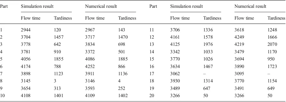
Discrete event simulation models using FlexSim software were constructed to evaluate the part dispatching sequence generated by the proposed approach. As in the numerical study, three performance indicators were employed to validate the results of the proposed method, namely flow time, tardi-ness, and makespan. The result of flow time and makespan can be acquired directly from the FlexSim simulation report. However, since tardiness is a derivation of flow time, it was calculated as the deviation between due date and acquired flow time. The results of both methods were compared to see the difference between them.
The main input for the simulation study was the schedule obtained by the proposed GA model, consisting of the arrival
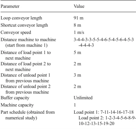
Fig. 7 Simulation model in FlexSim Table 9 Parameters of simulation model
Parameter Value
Loop conveyor length 91 m
Shortcut conveyor length 8 m
Conveyor speed 1 m/s
Distance machine to machine (start from machine 1)
3-4-4-3-3-5-5-4-6-5-4-5-6-4-5-3 -4-4-4-3
Distance of load point 1 to next machine
5 m
Distance of load point 2 to next machine
2 m
Distance of unload point 1 from previous machine
3 m
Distance of unload point 2 from previous machine
2 m
Buffer capacity Unlimited
Machine capacity 1
Part schedule (obtained from numerical study)
sequence and routing options of the parts. To compare the results of both methods, the simulation model study used the same parameter as used in the numerical study. The overall system was set to the same conditions as the numerical study, both on data sets (sequence, processing, and setup time) and layout properties (machine arrangement and travel distance). Table9summarizes the parameters of the simulation model.
An experimental example of the simulation study involved data set 5 since it is the most complex system in this study. The main element of this model was the loop conveyor, construct-ed using MergeSort in FlexSim. The shortcut was representconstruct-ed by two conveyors with opposite movement directions. The pick and drop points were placed along the MergeSort and connected to queues and machines, as well as loading and unloading points. The capacity of queue was assumed to be unlimited. Meanwhile, the machines have single capacity meaning they can only process one part at a time. Figure7 illustrates the example of simulation models on FlexSim. The results of the simulation experiment in FlexSim are presented in Table10.
Compared to the results of numerical study, there is a slight difference between both results. Generally, the value of the simulation result was somewhat lower than the numerical study result due to the different policy regarding the position-ing of pick and drop points. In the numerical study, it was assumed that both pick and drop point of each machine were positioned at the same point. Meanwhile, in the simulation study, there was a space between pick and drop points along
the conveyor. Nevertheless, the comparison indicated that both results are similar as depicted in Table11.
6 Conclusion
Effective and reliable model is critical for solving the re-entrant scheduling problems in FMS with consideration of the addition of multi loading-unloading points and turnta-ble shortcut into the loop layout configuration. As a solu-tion, a modified genetic algorithm was developed to gen-erate the near optimal solution. The crowding factor calcu-lated using the Euclidian distance was employed to mea-sure the population diversity of the generations. Substitu-tion based on the re-combinaSubstitu-tion and re-mutaSubstitu-tion was per-formed to modify the individuals with close similarity. A comparison study between the proposed approach and oth-er conventional methods showed that the proposed ap-proach exhibited better performance and robustness than conventional methods for both small and large datasets. The similarity analysis demonstrated that the proposed al-gorithm can tackle the population diversity issue by im-proving the crowding distance. Thus, the probability of obtaining near optimal solutions increases by avoiding ear-ly convergence.
Although increasing the complexity, the addition also offers alternative routes which can be shorter in distance than the current. The results of experiments with different designs indicated that the addition L/U stations and short-cut has significant effect in reducing the makespan, mean flow time, and total tardiness by cutting the traveling time of jobs. The outcomes of simulation confirmed that both studies were running alike and there were no errors in the numerical study computation. In future studies, it is worth considering the other variables to develop integrated FMS scheduling by combining the parts scheduling and vehicle
Table 11 Comparison of obtained objective functions value
Objective function Numerical Simulation Difference
Makespan 4252 4174 1.83 %
Mean flow time 3688 3686 0.05 %
Total tardiness 19,037 19,040 0.02 %
Table 10 Comparison of the result of simulation and numerical study
Part Simulation result Numerical result Part Simulation result Numerical result
Flow time Tardiness Flow time Tardiness Flow time Tardiness Flow time Tardiness
1 2944 120 2967 143 11 3706 1336 3618 1248
2 3704 1457 3717 1470 12 4161 1578 4249 1666
3 3778 642 3834 698 13 4125 1976 4219 2070
4 3781 910 3372 501 14 3342 1033 3479 1170
5 4056 1855 4086 1885 15 3770 1026 3694 950
6 4174 788 4252 866 16 3634 1467 3890 1723
7 3898 1123 3911 1136 17 3062 – 3095 –
8 3145 3 3146 4 18 3930 1314 3770 1154
9 3654 313 3593 252 19 3489 647 3491 649
routing as well as tool selection-allocation problems to constitute a complete scheduling system. It would also be interesting to investigate the relationship between the im-provement in productivity and investment cost of extra L/U stations and shortcut.
Acknowledgments The authors would like to acknowledge the Japan International Cooperation Agency (JICA) project of the ASEAN Univer-sity Network/the Southeast Asia Engineering Education Development Network (AUN/Seed-Net) and the Ministry of Higher Education for fi-nancial support under High Impact Research Grant UM.C/HIR/MOHE/ ENG/35 (D000035-16001).
Appendices
Appendix 1 Point to point distance
Table 12 Point to point distance
in case study 1 Stations L/U point M2 M6 M3 M1 M5 M4 M7
L/U point – 3 7 11 16 20 24 27
Shortcut 1 27 30 2 6 11 15 19 22
Shortcut 2 6 9 13 17 22 26 30 1
M2 29 – 4 8 13 17 21 24
M6 25 28 – 4 9 13 17 20
M3 21 24 28 – 5 9 13 16
M1 16 19 23 27 – 4 8 11
M5 12 15 19 23 28 – 4 7
M4 8 11 15 19 24 28 – 3
M7 5 8 12 16 21 25 29 –
Table 13 Point to point distance
in case study 2 Stations M1 M2 M3 M4 M5 M6 M7 M8 M9 M10
Central L/U 5 8 12 16 19 22 27 32 36 42
Extra load 40 43 2 6 9 12 17 22 26 32
Extra unload 16 19 23 27 30 33 38 43 2 8
Shortcut 1 36 39 43 2 5 8 13 18 22 28
Shortcut 2 21 24 28 32 35 38 43 3 7 13
M1 – 3 7 11 14 17 22 27 31 37
M2 42 – 4 8 11 14 19 24 28 34
M3 38 41 – 4 7 10 15 20 24 30
M4 34 37 41 – 3 6 11 16 20 26
M5 31 34 38 42 – 3 8 13 17 23
M6 28 31 35 39 42 – 5 10 14 20
M7 23 26 30 34 37 40 – 5 9 15
M8 18 21 25 29 32 35 40 – 4 10
M9 14 17 21 25 28 31 36 41 – 6
Table 14 Point to point distance
in case study 3 Stations M1 M2 M3 M4 M5 M6 M7 M8 M9 M10 M11 M12
Central L/U 5 8 12 16 19 22 27 32 36 42 47 51
Extra load 49 52 2 6 9 12 17 22 26 32 37 41
Extra unload 14 17 21 25 28 31 36 41 45 51 2 6
Shortcut 1 36 39 43 2 5 8 13 18 22 28 33 37
Shortcut 2 20 23 27 31 34 37 42 47 51 3 8 12
M1 – 3 7 11 14 17 22 27 31 37 42 46
M2 51 – 4 8 11 14 19 24 28 34 39 43
M3 47 50 – 4 7 10 15 20 24 30 35 39
M4 43 46 50 – 3 6 11 16 20 26 31 35
M5 40 43 47 51 – 3 8 13 17 23 28 32
M6 37 40 44 48 51 – 5 10 14 20 25 29
M7 32 35 39 43 46 49 – 5 9 15 20 24
M8 27 30 34 38 41 44 49 – 4 10 15 19
M9 23 26 30 34 37 40 45 50 – 6 11 15
M10 17 20 24 28 31 34 39 44 48 – 5 9
M11 12 15 19 23 26 29 34 39 43 49 – 4
M12 8 11 15 19 22 25 30 35 39 45 50 –
Table 15 Point to point distance in case study 4
Stations M1 M2 M3 M4 M5 M6 M7 M8 M9 M10 M11 M12 M13 M14 M15
Central L/U 5 13 20 27 36 43 50 57 64 66 72 78 86 92 98
Extra load 74 82 89 96 3 10 17 24 31 33 39 45 53 59 65
Extra unload 25 33 40 47 56 63 70 77 84 86 92 98 4 10 16
Shortcut 1 84 92 99 4 13 20 27 34 41 43 49 55 63 69 75
Shortcut 2 25 33 40 47 56 63 70 77 84 86 92 98 4 10 16
M1 – 8 15 22 31 38 45 52 59 61 67 73 81 87 93
M2 94 – 7 14 23 30 37 44 51 53 59 65 73 79 85
M3 87 95 – 7 16 23 30 37 44 46 52 58 66 72 78
M4 80 88 95 – 9 16 23 30 37 39 45 51 59 65 71
M5 71 79 86 93 – 7 14 21 28 30 36 42 50 56 62
M6 64 72 79 86 95 – 7 14 21 23 29 35 43 49 55
M7 57 65 72 79 88 95 – 7 14 16 22 28 36 42 48
M8 50 58 65 72 81 88 95 – 7 9 15 21 29 35 41
M9 43 51 58 65 74 81 88 95 – 2 8 14 22 28 34
M10 41 49 56 63 72 79 86 93 100 – 6 12 20 26 32
M11 35 43 50 57 66 73 80 87 94 96 – 6 14 20 26
M12 29 37 44 51 60 67 74 81 88 90 96 – 8 14 20
M13 21 29 36 43 52 59 66 73 80 82 88 94 – 6 12
M14 15 23 30 37 46 53 60 67 74 76 82 88 96 – 6
Appendix 2 Layout of the systems
Table 16 Point to point distance in case study 5
Stations M1 M2 M3 M4 M5 M6 M7 M8 M9 M10 M11 M12 M13 M14 M15 M16 M17 M18 M19 M20
Central L/U 5 8 12 16 19 22 27 32 36 42 47 51 56 62 66 71 74 78 82 86
Extra load 74 77 81 85 88 2 7 12 16 22 27 31 36 42 46 51 54 58 62 66
Extra unload 18 21 25 29 32 35 40 45 49 55 60 64 69 75 79 84 87 2 6 10
Shortcut 1 77 80 84 88 2 5 10 15 19 25 30 34 39 45 49 54 57 61 65 69
Shortcut 2 22 25 29 33 36 39 44 49 53 59 64 68 73 79 83 88 2 6 10 14
M1 – 3 7 11 14 17 22 27 31 37 42 46 51 57 61 66 69 73 77 81
M2 86 – 4 8 11 14 19 24 28 34 39 43 48 54 58 63 66 70 74 78
M3 82 85 – 4 7 10 15 20 24 30 35 39 44 50 54 59 62 66 70 74
M4 78 81 85 – 3 6 11 16 20 26 31 35 40 46 50 55 58 62 66 70
M5 75 78 82 86 – 3 8 13 17 23 28 32 37 43 47 52 55 59 63 67
M6 72 75 79 83 86 – 5 10 14 20 25 29 34 40 44 49 52 56 60 64
M7 67 70 74 78 81 84 – 5 9 15 20 24 29 35 39 44 47 51 55 59
M8 62 65 69 73 76 79 84 – 4 10 15 19 24 30 34 39 42 46 50 54
M9 58 61 65 69 72 75 80 85 – 6 11 15 20 26 30 35 38 42 46 50
M10 52 55 59 63 66 69 74 79 83 – 5 9 14 20 24 29 32 36 40 44
M11 47 50 54 58 61 64 69 74 78 84 – 4 9 15 19 24 27 31 35 39
M12 43 46 50 54 57 60 65 70 74 80 85 – 5 11 15 20 23 27 31 35
M13 38 41 45 49 52 55 60 65 69 75 80 84 – 6 10 15 18 22 26 30
M14 32 35 39 43 46 49 54 59 63 69 74 78 83 – 4 9 12 16 20 24
M15 28 31 35 39 42 45 50 55 59 65 70 74 79 85 – 5 8 12 16 20
M16 23 26 30 34 37 40 45 50 54 60 65 69 74 80 84 – 3 7 11 15
M17 20 23 27 31 34 37 42 47 51 57 62 66 71 77 81 86 – 4 8 12
M18 16 19 23 27 30 33 38 43 47 53 58 62 67 73 77 82 85 – 4 8
M19 12 15 19 23 26 29 34 39 43 49 54 58 63 69 73 78 81 85 – 4
M20 8 11 15 19 22 25 30 35 39 45 50 54 59 65 69 74 77 81 85 –
(i) Layout in case study 1
Fig. 8
(ii) Layout in case study 2
Fig. 9
(iii) Layout in case study 3
References
1. Chan FT, Swarnkar R (2006) Ant colony optimization approach to a fuzzy goal programming model for a machine tool selection and operation allocation problem in an FMS. Robot Comput Integr Manuf 22(4):353–362
2. Kumar RS, Asokan P, Kumanan S (2009) Artificial immune system-based algorithm for the unidirectional loop layout problem in a flexible manufacturing system. Int J Adv Manuf Technol 40(5– 6):553–565
3. Ozcelik F, Islier AA (2011) Generalisation of unidirectional loop layout problem and solution by a genetic algorithm. Int J Prod Res 49(3):747–764
4. Hall NG, Sriskandarajah C, Ganesharajah T (2001) Operational decisions in AGV-served flowshop loops: scheduling. Ann Oper Res 107(1–4):161–188
5. Gamila MA, Motavalli S (2003) A modeling technique for loading and scheduling problems in FMS. Robot Comput-Integr Manuf 19(1):45–54
6. Zeballos L, Quiroga O, Henning GP (2010) A constraint program-ming model for the scheduling of flexible manufacturing systems with machine and tool limitations. Eng Appl Artif Intell 23(2):229– 248
7. MacCarthy B, Liu J (1993) A new classification scheme for flexible manufacturing systems. Int J Prod Res 31(2):299–309
8. Haq AN, Karthikeyan T, Dinesh M (2003) Scheduling decisions in FMS using a heuristic approach. Int J Adv Manuf Technol 22(5–6): 374–379
9. Keung K, Ip W, Yuen D (2003) An intelligent hierarchical work-station control model for FMS. J Mater Process Technol 139(1): 134–139
10. Das SR, Canel C (2005) An algorithm for scheduling batches of parts in a multi-cell flexible manufacturing system. Int J Prod Econ 97(3):247–262
11. Sankar SS, Ponnambalam S, Gurumarimuthu M (2006) Scheduling flexible manufacturing systems using parallelization of multi-objective evolutionary algorithms. Int J Adv Manuf Technol 30(3–4):279–285
12. Jerald J, Asokan P, Saravanan R, Rani ADC (2006) Simultaneous scheduling of parts and automated guided vehicles in an FMS en-vironment using adaptive genetic algorithm. Int J Adv Manuf Technol 29(5–6):584–589
13. Huang R-H, Yu S-C, Kuo C-W (2014) Reentrant two-stage multi-processor flow shop scheduling with due windows. Int J Adv Manuf Technol 71(5–8):1263–1276
14. Jeong B, Kim Y-D (2014) Minimizing total tardiness in a two-machine re-entrant flowshop with sequence-dependent setup times. Comput Oper Res 47:72–80
15. Burnwal S, Deb S (2013) Scheduling optimization of flexible manufacturing system using cuckoo search-based approach. Int J Adv Manuf Technol 64(5–8):951–959
16. Souier M, Sari Z, Hassam A (2013) Real-time rescheduling metaheuristic algorithms applied to FMS with routing flexibility. Int J Adv Manuf Technol 64(1–4):145–164
17. Joseph O, Sridharan R (2011) Analysis of dynamic due-date assign-ment models in a flexible manufacturing system. J Manuf Syst 30(1):28–40
18. Cardin O, Mebarki N, Pinot G (2013) A study of the robustness of the group scheduling method using an emulation of a complex FMS. Int J Prod Econ 146(1):199–207
19. Udhayakumar P, Kumanan S (2012) Integrated scheduling of flex-ible manufacturing system using evolutionary algorithms. Int J Adv Manuf Technol 61(5–8):621–635
20. Hsu T, Korbaa O, Dupas R, Goncalves G (2008) Cyclic scheduling for FMS: modelling and evolutionary solving approach. Eur J Oper Res 191(2):464–484
21. Qin W, Zhang J, Sun Y (2013) Multiple-objective scheduling for interbay AMHS by using genetic-programming-based composite dispatching rules generator. Comput Ind 64(6):694–707
22. Caridá V, Morandin Jr O, Tuma C (2015) Approaches of fuzzy systems applied to an AGV dispatching system in a FMS. Int J Adv Manuf Technol:1–11
23. Chan FT, Chung S, Chan P An introduction of dominant genes in genetic algorithm for scheduling of FMS. In: Intelligent Control, 2005. Proceedings of the 2005 I.E. International Symposium on, Mediterrean Conference on Control and Automation, 2005. IEEE, pp 1429–1434
24. Chan F, Chung S, Chan P (2006) Application of genetic algorithms with dominant genes in a distributed scheduling problem in flexible manufacturing systems. Int J Prod Res 44(3):523–543
25. Chan FT, Chung S, Chan L, Finke G, Tiwari M (2006) Solving distributed FMS scheduling problems subject to maintenance: genetic algorithms approach. Robot Comput Integr Manuf 22(5):493–504
(iv) Layout in case study 4
Fig. 11
(v) Layout in case study 5
26. Mejía G, Odrey NG (2006) An approach using Petri Nets and im-proved heuristic search for manufacturing system scheduling. J Manuf Syst 24(2):79–92
27. Lee J, Lee JS (2010) Heuristic search for scheduling flexible manufacturing systems using lower bound reachability matrix. Comput Ind Eng 59(4):799–806
28. Hsu T, Dupas R, Goncalves G A genetic algorithm to solving the problem of flexible manufacturing system cyclic scheduling. In: Systems, Man and Cybernetics, 2002 I.E. International Conference on, 2002. IEEE, p 6 pp. vol. 3
29. Sun Y, Zhang C, Gao L, Wang X (2011) Multi-objective optimiza-tion algorithms for flow shop scheduling problem: a review and prospects. Int J Adv Manuf Technol 55(5–8):723–739
30. Prakash A, Chan FT, Deshmukh S (2011) FMS scheduling with knowledge based genetic algorithm approach. Expert Syst Appl 38(4):3161–3171
31. Ebrahimi M, Fatemi Ghomi S, Karimi B (2014) Hybrid flow shop scheduling with sequence dependent family setup time and uncer-tain due dates. Appl Math Model 38(9):2490–2504
32. Chan FT, Chan HK (2004) A comprehensive survey and future trend of simulation study on FMS scheduling. J Intell Manuf 15(1):87–102
33. Low C, Yip Y, Wu T-H (2006) Modelling and heuristics of FMS scheduling with multiple objectives. Comput Oper Res 33(3):674– 694
34. Low C, Wu T-H (2001) Mathematical modelling and heuristic ap-proaches to operation scheduling problems in an FMS environment. Int J Prod Res 39(4):689–708
35. Baruwa OT, Piera MA (2014) Anytime heuristic search for sched-uling flexible manufacturing systems: a timed colored Petri net approach. Int J Adv Manuf Technol 75(1–4):123–137
36. Zhou R, Nee A, Lee H (2009) Performance of an ant colony opti-misation algorithm in dynamic job shop scheduling problems. Int J Prod Res 47(11):2903–2920
37. Renna P (2010) Job shop scheduling by pheromone approach in a dynamic environment. Int J Comput Integr Manuf 23(5):412–424 38. Zhao F, Jiang X, Zhang C, Wang J (2014) A chemotaxis-enhanced
bacterial foraging algorithm and its application in job shop sched-uling problem. Int J Comput Integr Manuf (ahead-of-print):1–16 39. Kim K, Yamazaki G, Lin L, Gen M (2004) Network-based hybrid
genetic algorithm for scheduling in FMS environments. Artif Life Intell 8(1):67–76
40. Godinho Filho M, Barco CF, Neto RFT (2012) Using Genetic Algorithms to solve scheduling problems on flexible manufacturing systems (FMS): a literature survey, classification and analysis. Flex Serv Manuf J:1–24
41. Reeves CR, Rowe JE (2003) Genetic algorithms: principles and perspectives: a guide to GA theory, vol 20. Springer, Dordrecht 42. Chen J-S, Pan JC-H, Lin C-M (2008) A hybrid genetic algorithm
for the re-entrant flow-shop scheduling problem. Expert Syst Appl 34(1):570–577
43. Deb K, Pratap A, Agarwal S, Meyarivan T (2002) A fast and elitist multiobjective genetic algorithm: NSGA-II. IEEE Trans Evol Comput 6(2):182–197
44. Barnes J, Laguna M (1991) A review and synthesis of tabu search applications to production scheduling problems. ORP91-05 45. Brandimarte P (1993) Routing and scheduling in a flexible job shop
by tabu search. Ann Oper Res 41(3):157–183