A wave matrix
Andrew Brody
Institute of Economics,Budao¨rsi u´t 45,1112 Budapest, Hungary
Abstract
A wave matrix is presented consisting of price and quantity elasticities. Its eigenvalues determine the feasible cycles of a dynamic Leontief system. A numerical illustration and a 20-year trajectory are computed with the aid of a seven sector USA matrix for the year 1958. A short discussion of further work required closes the paper. © 2000 Elsevier Science B.V. All rights reserved.
JEL classification:C67; E37
Keywords:Growth; Cycles; Elasticities; Forecasting
1. Introduction
Richard Goodwin’s late research brought a fusion of the linear Leontief system with his own logarithmic growth theory1. In Goodwin (1989) he then showed the
possible fluctuations of an input – output system around a non-focal, not attracting equilibrium path. A similar non-linear system of differential equations is investi-gated, proposed in Brody (1989). The basic task of the paper is to find a suitable linear approximation to an extended dynamic Leontief system, in which the realized rates of profit determine expansion and the relative disequilibrium of markets governs price formation. The approximation involves two steps to handle the nonlinearity. The first is an exact reduction to stationary quantities, the second is an approximation that does not seriously distort the motion while the system remains in the vicinity of the equilibrium path.
E-mail address:[email protected] (A. Brody).
1Goodwin (1967). This is a variant of the ecological models of Volterra and Lotka. It may be also
considered as a mathematical restatement of Marx’s cycle theory.
In the next section thus an input – output ‘wave matrix’ is constructed to model economic cycles. It is linearized around the equilibrium von Neumann Ray of the system. In the third section some illustrative numerical results are presented and a 20-year forecast, based on USA data for 1958, is exhibited and discussed.
2. Construction of the wave matrix
The proposed system of cross regulation, where markets act on prices in the first equation, and profits determine growth in the second, has been set up by starting from simple accounting identities2
. It is a skew-symmetric dual system.
Price changes (the logarithmic derivatives of thepprices) are governed by excess demand:
while expansion of outputs (the logarithmic derivatives of theq quantities) depend on the rate of profits:
Hereaik are the flow andbik the stock coefficients of the Input – Output system.
In the first equation the market surplus is divided by total capital. In the second the apparent profit is divided with capital intensity.
It is well known3 that such a system permits a positive equilibrium path, the so
called von Neumann Ray. The economic interpretation of this solution is not strictly symmetric. It implies constant prices but growing quantities. To circumvent this theoretical asymmetry in the definition we reduce the quantities to render their equilibrium values constant. This can be done by continuously ‘discounting’ them with the uniform equilibrium growth rate. Thus instead of the (possibly non-equi-librium) quantitiesqi, we take their transforms
xi=exp(−lt)qi (2)
We may assume, without loss of generality, that at the initial momentt=0. At
t=0 the two quantities coincide, and the reduction is exact. Essentially, we split changes in q into two components, an equilibrium growth rate and a fluctuation around the growth path. By focusing on x instead onq we explain the deviations from the equilibrium growth rate l.
2The model may be considered also as an ensemble of stylized uniform behavioral equations or be
deduced from extreme conditions of long run maximization.
3The first proof has been furnished by Neumann (1937) and Neumann (1945). The dynamic theory
This transformation requires us to augment the matrix of flow coefficients with the stock coefficients, the latter multiplied by the equilibrium rate. Thus the equilibrium ray is turned into a singularity of the governing equation. To do this in a transparent manner we change to matrix notation. We then need theA={aik}
flow and B={bik} stock matrices. From these the equilibrium price, p¯, and
quantity, x¯, vectors are computed4 as the left and right hand eigenvectors of the
matrixA+lB.The vectors x¯andq¯, are then the same eigenvectors, connected, as they are, by a (growing) scalar multiplier.
p¯%=p¯%A+lp¯%B (3)
and
x¯=Ax¯+lBx¯ (3b)
Let us now denote the full von Neumann Ray by forming the z¯ vector as the concatenation of the equilibrium vectorsp¯andx¯. The firstnelements are the prices, the second n elements the quantities.
z¯%=[p¯%,x¯%], and also generally z%=[p%,x%] (4)
The corresponding hyper-matrix of the right hand (extended flow) coefficients is skew-symmetric. When postmultiplied by a possibly non-equilibrium vector z it expresses the (positive ore negative) absolute deviations. These are the positive (or negative) excess demands and the sectoral surpluses (or deficits) of profits over (or under) their equilibrium amount. Let us denote this matrix by the letter K,
habitually used for skew-symmetric matrices.
K=
0 A+lB−11−A%−lB% 0
(5)Kz=0 if and only ifz=z¯, the von Neumann Ray, on account of the definitional equations (3) and (4).
In a linear model the left hand stock hyper-matrix (acting on absolute changes) consists of the usual stock matrices to be multiplied by the differential ofz.
D=
0 BB% 0
(6)It would thus contain the symmetrically arranged stock matrices on which the changes themselves act. But we have to handle the non-linearity. It is not directly the amount of excess, but its relative rate that triggers the changes. We also seek the change as a logarithmic differentialz;/z. We thus require rates of change. A profit rate, that is computed by dividing excess profits by capital intensities, and a rate of price changes, that may be computed by dividing excess demand by the total marketable, that is: existing amount of the respective commodities and services.
4The value of the equilibrium growth and profit rate,l, is best calculated as the reciprocal of the
unique, dominant and positive eigenvalue of the strictly positive matrixQB. HereQ=(1−A)−1is the
These proportionalities are furnished by the divisors on the left and the right side in the dual system of Eq. (1) and Eq. (1b). In matrix form they may be collected into the main diagonal of the left hand hyper-matrix. The complete (non-linear) left hand hyper-matrix may be written out as
S=diagDz./z−D (7)
Here we use a capital S, habitually used for symmetric matrices. Thus, as can be seen, the matrixSremains symmetric even after the inclusion of the main diagonal that carries the non-linear ‘disturbance’ of the linear system. The operation ‘./’ designates an element by element division of the respective vectors. The dynamic system thus reads simply as
Sz;=Kz (8)
but it is nonlinear, because the main diagonal of the left hand matrix still depends explicitly onz according to Eq. (7).
The trick that effects the linearization of the matrixSis to neglect its dependence on actual, never exactly equilibrium, prices and quantities by substituting, instead, their equilibrium values:
S=diagDz¯./z¯−D (7b)
We shall show later that the exact and the linearized solutions almost coincide and their spectra (the cyclic frequencies) are the same as long as we remain close to equilibrium.
But one problem still remains. The matrix S (both in its original and in its linearized form) is singular. It can not be inverted in the usual sense. Yet it has the same null space as the matrixK, that is: on the von Neumann ray Szequals zero. As we are interested only in the non-equilibrium motion of the system, we may safely use a so called pseudo-inversion. In a pseudo-inversion the diads pertaining to zero eigenvalues are neglected and only the reciprocals of the (here positive) other eigenvalues are considered in the process of inversion.
The system 8 thus has a zero eigenvalue5, belonging to the equilibrium path.
Besides this it possesses only purely imaginary eigenvalues, the cyclic frequencies, generating orbits around the von Neumann Ray. The system matrix is thus similar to a skew-symmetric matrix that has only zero and imaginary eigenvalues. An additional trick, a further similarity transformation, renders the system matrix measure-invariant. Let us designate by the letter Z (capital Z) a diagonal matrix with its diagonal occupied by the von Neumann Ray:
Z=diagz¯ (9)
We will call the matrix W the wave matrix of the system, if it is of the form
5More precisely: it has two zero eigenvalues, one for equilibrium prices and one for equilibrium
W=Z−1 S−1
K Z (10)
The inversion ofSis to be performed as a pseudo-inversion, as explained above. The wave matrix W is thus a similarity transform of the system matrix of the differential Eq. (8) and it
1. has a zero trace (the elements on its main diagonal add up to zero),
2. has all its row sums equal to zero (adding the elements in a row amounts to postmultiplying the matrix with its equilibrium vector),
3. produces a zero vector if premultiplied by the squared elements of z (for the same reason).
From these facts we conclude that the changes (and thus all cyclic trajectories) are perpendicular to the equilibrium vector. The scalar valuez’zremains constant on the (cyclic) path.
The similarity transformation by the matrixZserves to translate the equilibrium point to a vector of unit magnitudes. We may therefore consider the elements of this matrix W, that exhibit the non-equilibrium response triggered by a non equilibrium state (or triggered by any perturbation of the equilibrium), both as absolute or relative deviations. The main force of Goodwin’s approach — working with pure numbers without dimension, scale-free elasticities — is maintained and may be exploited when interpreting the numerical illustration presented below.
3. Numerical results
3.1.Data and growth rate
To illustrate such a wave matrix, the system was implemented with the data used to compute equilibrium quantities and growth rate for the United States in Brody (1966). Appendix A lists the basic data: a seven-order 1958 flow coefficient matrix and approximate product life-spans for each sector, used to estimate a capital coefficient, or stock, matrix.
While the data were very crude the early computations produced quite reasonable results. In particular, the equilibrium growth rates (computed in 1964 at the Harvard Economic Research Project) were close to 4%, comparing well with the average rate6 observed over the next 20 years from 1959 to 1978. Input-output
computation do have an error-correcting facet. Even if the flow coefficients (and thus also the eigenvectors) are correct only in their first digit, the eigenvalues already possess a 2-digit precision. Nevertheless this peculiarity holds only for the synthetic, average, aggregated or macroeconomic indices. Thus one may expect dependable results only for the computed cyclic frequencies, that is cycle-lengths, not for all the results7
. The error of the price and quantity elasticities, some of
7This peculiar but very useful fact is granted by the theory of the Raleigh – Aitken quotient. See
Bodewig (1952).
6For the 1960s, average growth stood slightly above this mark but it did drop below 4% during the
which will be presented below, are strongly affected by the probably sizable errors of the original data.
3.2.Elasticities
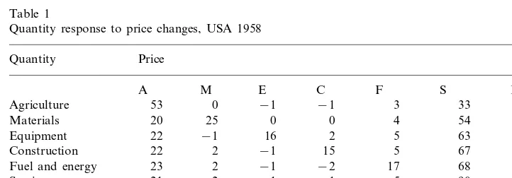
The elements of the wave matrix are measure-invariant and therefore also all the eigenvalues. In Table 1 only the third quadrant of the matrix is exhibited. This is the quantity response (by branches indicated in the rows) triggered by an increase in the price of the respective branches (set out columnwise).
This quadrant (see Table 1) as a matrix, is always positive semidefinite but not all of its off-diagonal elements are negative. It is interesting to see that agricultural and service-sector price increases are associated with increases in the outputs of most other sectors. The years 1959 – 78 actually witnessed a very rapid autonomous, self-boosting growth of services.
An increase of wages seems to uniformly lower output in all other sectors. Households, on the other hand, respond most sensitively to increases in agricultural and service prices, less so to those of other sectors. Household is also the only sector that seemingly had an own quantity/price elasticity \1. Equipment and construction prices do not seem to affect other branches.
Given the crudeness of the data and the simplified behavioral assumptions, we should not attribute too much significance to the actual size of these first estimates of individual elasticities. The response of the household sector seems to be also particularly exaggerated. This abrupt reaction may stem from a conceptual fault in the data: a very small stock multiplier, used for the household row8. This part of
Table 1
Quantity response to price changes, USA 1958 Price
8The neglect of human capital-in tabulations and otherwise-seems to be a constant source of
the computation should yield much clearer results when a more realistic, or actual, stock matrix is used instead of our makeshift one. But, alas, I did not yet find detailed and good stock data and my results for perturbation (or sensitivity) analysis are also very meager for the time being.
The 2nd quadrant, not presented here, the response of prices on oversupply, proved to be negative semidefinite, as expected. It has a dominant negative diagonal but the other elements were not all positive. The 1st and 4th quadrants (price/price and quantity/quantity elasticities) are of minor importance, but they do exist and will have to be inspected more closely when better data warrant the exercise.
3.3.Frequencies
The (purely imaginary) eigenvalues of the wave matrix are, in increasing order (rounded to two decimals)
v=0 0.1 0.23 0.34 0.90 1.2 8.9
The feasible cycle-lengths, computed as T=2p/v (rounded to years) are thus:
T= 65 27 19 7 5 1
Thus the Kondratiev wave, the demographic (generational) swing, an equipment or building cycle, two shorter inventory cycles and a yearly seasonality are already in the repertory of this simple model. If we search the actual GDP series from 1959 to 1978 we may find power-peaks only for the 5, 7 and 19 year cyclic components. Neither the short cycle nor the longer ones are discernible in the relatively short time series. But other evidence suggests that they do exist and may be found in the longer series9
.
3.4.Forecasting
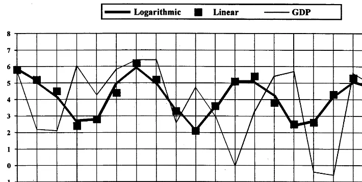
The next step is to compare actual annual GDP growth rates with those computed on the basis of this model. Both the logarithmic and linear model were computed with second and third order Runge – Kutta formulas to 4 digit precision. This level is more than adequate for illustrative purposes because the resolving power of most graphs does not exceed a 3 digit precision.
In Fig. 1, the results of the linear approximation are very close to the exact logarithmic trajectory. They are, for practical purposes, hardly discernible from the latter. Considering that economists normally accept a 2-digit accuracy in estimating growth rates, it is permissible to consider the two systems as virtually equivalent. The same is also true for the details of the computation (sectoral prices and quantities), not presented here.
9Quarterly data for the same period do show short fluctuations and also a relative maximum of
Fig. 1. Computed and actual growth rates. The GDP growth data were copied from the NIPA homepage.
This comes as no surprise. In spite of their jagged outline, the trajectories do not deviate more than a few percentage points above and below their average. There-fore the ‘bias’ of the linear approximation did not reach a1
2% magnitude even in the
worst cases. Moreover, because of the periodic character of the trajectory, the deviations do not accumulate; thus the linear approximation is and stays close to the logarithmic path.
Nevertheless the forecasting power of the model is less than impressive. Though the computed path for the 20 years exhibits a very high correlation with the actual one (R2=0.99), computed and actual yearly growth rates correlate much less well
and show an increasingly deviating pattern. Fluctuations in the overall level of economic performance grew strongly in the 1970s. There were two heavy recessions, with troughs registered in November 1970 and March 1975, the latter attributed to the world-wide oil crisis. They are not reflected by the computation. For the second decade the whole exercise ceases to be meaningful, even if producing the closest fit, by sheer chance, for the latter years.
No account was taken of monetary and fiscal intervention of the government, taxation and subsidies that might change significantly the conditions of supply and demand. Intervention, besides changing often quite abruptly, is mostly displaying a Sisyphean character. It apparently can not dispense with cycles. In the best case it may roll them away, perhaps even attenuate some of them, presumably the minor ones, only to find them coming back, sometimes with increased amplitudes. The intensification of fluctuations in the 1970s is well known, much discussed in the pertinent literature and shown in the actual data of the graph.
4. Conclusion
The idea of cross-regulation, prices acting on quantities and quantities on prices, enunciated and explained more than 2 centuries ago by Adam Smith seems to work quite well in a qualitative sense. It explains equilibrium, growth, and also fluctua-tions around the equilibrium path of growth. In its modern mathematical form, as engineered by Neumann, Leontief, Goodwin and implemented by up to date statistical findings, it allows for assessment of the long-run growth and the feasible (observable) cycle lengths, and also their general amplitude fairly well.
The questions of individual phasing and amplitude remain still open, and with it the merits and pitfalls of government intervention. The wave matrix, presented in this paper, offers a contemporary framework for linking the time profiles of macro and sectoral fluctuation in outputs and prices with the basic structural proportions represented in dynamic input – output systems.
The computations presented here were based on very crude data for the USA and compared the solutions with observed time series. The results, while hardly final or overly impressive, suggest that the age old approach is still progressive and promising. It also verifies that Goodwin’s pioneering logarithmic model may be well approximated by an aptly chosen linear system that has a closed solution and permits analytical results. Further computations using more detailed and more realistic data, particularly in the area of capital coefficients and household labor supply, should bring the results better into line with observed economic reality. The approach, suggested in this paper, sets out an ambitious agenda of further empirical and theoretical work. Sensitivity testing, inclusion of money and taxation, government policy intervention and the mathematical analysis of the characteristi-cally different branch profiles of the cycles of short, medium and long duration seem to be the next steps. It can only be hoped that this classical subject still generates sufficient interest to get that work going.
Acknowledgements
Appendix A
The HERP flow matrix for the USA 195810
0.0619 0.2778
Bodewig, J., 1952. Matrix Calculus. North Holland, Amsterdam. Brody, A., 1966. A Simplified Growth Model. Q. J. Econ. (80).
Brody, A., 1989. Growth cycles in economics. In: Casti-Karlquist, Newton to Aristotle, Toward a Theory of Models for Living Systems. Birkha¨user, Basel.
Goodwin, R., 1967. A growth cycle. In: Feinstein (Ed.). Socialism, Capitalism and Economic Growth. Cambridge University Press, Cambridge.
Goodwin, R., 1989. Swinging along the autostrada: cyclical fluctuations along the von Neumann Ray. In: Dore, Chakravarty, Goodwin (Eds). John von Neumann and Modern Economics. Clarendon Press, Oxford.
Leontief, W., et al., 1953. Studies in the Structure of American Economy. Oxford University Press, New York.
Neumann, J., 1937. U8ber ein o¨konomisches gleichungssystem und eine verallgemeinerung des brouwer-schen fixpunktsatzes. Ergeb. Math. Colloq. 8, 73 – 83.
Neumann, J., 1945. A model of general economic equilibrium. Rev. Econ. Stud. 13, 1 – 9.
10The flow matrix has been furnished by the USA Department of Commerce, Bureau of Economic
Analysis. It has been cross checked and aggregated by the Harvard Economic Research Project.
11In the 1964 computation this multiplier had been assumed to be zero. Here an approximately half