What You Need to Know about
Machine Learning
Leveraging data for future telling and data analysis
Gabriel Cánepa
What You Need to Know about Machine
Learning
Copyright © 2016 Packt Publishing
All rights reserved. No part of this book may be reproduced, stored in a retrieval system, or transmitted in any form or by any means, without the prior written permission of the publisher, except in the case of brief quotations embedded in critical articles or reviews. Every effort has been made in the preparation of this book to ensure the accuracy of the information presented. However, the information contained in this book is sold without warranty, either express or implied. Neither the author, nor Packt Publishing, and its dealers and distributors will be held liable for any damages caused or alleged to be caused directly or indirectly by this book.
Packt Publishing has endeavored to provide trademark information about all of the companies and products mentioned in this book by the appropriate use of capitals. However, Packt Publishing cannot guarantee the accuracy of this information. First published: November 2016
Production reference: 1181116
Published by Packt Publishing Ltd. Livery Place
35 Livery Street Birmingham B3 2PB, UK.
About the Author
Gabriel Cánepa is a Linux Foundation Certified System Administrator
www.PacktPub.com
For support files and downloads related to your book, please visit www.PacktPub.com. Did you know that Packt offers eBook versions of every book published, with PDF and ePub files available? You can upgrade to the eBook version at www.PacktPub.com and as a print book customer, you are entitled to a discount on the eBook copy. Get in touch with us at [email protected] for more details.At www.PacktPub.com, you can also read a collection of free technical articles, sign up for a range of free newsletters and receive exclusive discounts and offers on Packt books and eBooks.
https://www.packtpub.com/mapt
Get the most in-demand software skills with Mapt. Mapt gives you full access to all Packt books and video courses, as well as industry-leading tools to help you plan your personal development and advance your career.
Why subscribe?
Fully searchable across every book published by Packt Copy and paste, print, and bookmark content
Table of Contents
Section 1
: Types of Machine Learning
4Supervised learning 4
Unsupervised learning 6
Reinforcement learning 6
Reviewing machine-learning types 6
Section
2: Algorithms and Tools
9Introducing the tools 9
Installing the tools 10
Installation in Microsoft Windows 7 64-bit 11
Installation in Linux Mint 18 (Mate desktop) 64-bit 15
Exploring a well-known dataset for machine learning 19
Training models and classification 21
Section
3: Machine Learning and Big Data
25The challenges of big data 25
The first V in big data – volume 26
The second V – variety 27
The third V – velocity 27
Introducing a fourth V – veracity 28
Why is big data so important? 29
MapReduce and Hadoop 30
Section
4: SPAM Detection - a Real-World Application of Machine
Overview
It is a well-established fact that we, as human beings, learn through experience. During our early childhood, we learn to imitate sounds, form words, group them into phrases, and finally how to talk to another person. Later, in elementary school, we are taught numbers and letters, how to recognize them, and how to use them to make calculations and spell words. As we grow up, we incorporate these lessons into a wide variety of real-lifesituations and circumstances. We also learn from our mistakes and successes, and then use them to create strategies for decision making that will result in better performance in our daily lives. Similarly, if a machine--or more accurately, a computer program--can improve how it performs a certain task based on past experience, then you can say that it has learned or that it has extracted knowledge from data.
The term machine learning was first defined by Arthur Samuel in 1959 as follows:
Machine learning is the field of study that gives computers the ability to learn without being explicitly programmed.
Based on that definition, he developed what later became known as the Samuel's checkers-player algorithm, whose purpose was to choose the next move based on a number of factors (the number and position of pieces--including kings--on each side). This algorithm was first executed by an IBM computer, which incorporated successful and winning moves into its program, and thus learned to play the game through experience. In other words, the
computer learned winning strategies by repeatedly playing the game. On the other hand, a regular Checkers game that is set up with traditional programming cannot learn and
Overview
[ 2 ]
As opposed to traditional learning (where a program and input data are fed into a
computer to produce a desired output or result), machine learning focuses on the study of algorithms that help improve the performance of a given task through experience--meaning executions or runs of the same program. In other words, the overall goal is the design of computer programs that can learn from data and make predictions based on that learning. As we will discover throughout this book, machine learning has strong ties with statistics and data mining and can assist in the process of summarizing data for analysis, prediction (also known as regression), and classification. Thus, businesses and organizations using machine learning tools have the ability to extract knowledge from that data in order to increase revenue and human productivity or reduce costs and human-related losses. In order to effectively use machine learning, keep in mind that you must start with a question in mind. For example, how can I increase the revenue of my business? What seem to be the browsing tendencies among the visitors to my website? What are the main products bought by my clients and when? Then, by analyzing the associated data with the help of a trained machine, you can take informed decisions based on the predictions and classifications provided by it. As you can see, machine learning does not free you from taking actions but gives you the necessary information to ensure those actions are properly supported by thorough analysis.
What You Need to Know about
Machine Learning
This eGuide is designed to act as a brief, practical introduction to machine learning. It is full of practical examples which will get you up a running quickly with the core tasks ofmachine learning.
We assume that you know a bit about what machine learning is, what it does, and why you want to use it, so this eGuide won’t give you a history lesson in the background of machine learning. What this eGuide will give you, however, is a greater understanding of the key basics of machine learning so that you have a good idea of how to advance after you’ve read the guide. We can then point you in the right direction of what to learn next after giving you the basic knowledge to do so.
What You Need to Know about Machine Learning will:
Cover the fundamentals and the things you really need to know, rather than niche or specialized areas.
Assume that you come from a fairly technical background and so understand what the technology is and what it broadly does.
Focus on what things are and how they work.
1
Types of Machine Learning
Machine learning can be classified into three categories based on the characteristics of the data that is provided and the training methodology:Supervised learning Unsupervised learning Reinforcement learning
Let's examine each of them in detail.
Supervised learning
With supervised learning, the machine is trained using a set of labeled data, where each element is composed of given input/outcome pairs. The machine learns the relationship between the input and the outcome, and the goal is to predict behavior or make a decision based on previously given data. For example, we can provide the machine with the following input to get specific specific outcomes:
A set of integer numbers (or letters), and then train it to recognize a handwritten number or letter.
A set of musical notes, and then teach it to recognize the name and the associated pitch.
Types of Machine Learning
[ 5 ]
A list of web-browsing habits, and then teach it to provide search suggestions accordingly. A person whose web searches are mostly related to traveling will get somewhat different results than the individual who often looks for training opportunities when they enter the word train in an online search engine.
In the preceding examples, keep in mind that you need to label your data before feeding it to the machine. In the example of the movie list, let's consider a rather small dataset with two individuals named, A and B:
Individual Movies watched
A Harry Potter and the Philosopher's Stone
A Harry Potter and the Prisoner of Azkaban
B Star Wars: Episode IV – A New Hope A Harry Potter and the Order of the Phoenix
B The Empire Strikes Back
B Star Wars: Episode VI – Return of the Jedi A Harry Potter and the Deathly Hallows – Part 1 B Star Wars: Episode I – The Phantom Menace
Based on the preceding data, we can infer that individual A is a Harry Potter fan (perhaps he's also a fan of fantasy films as well), whereas B enjoys Star Wars movies (possibly science fiction as well). The answers to questions such as will individual A like “Harry Potter and the
Chamber of Secrets” or “Percy Jackson & the Olympians: The Lightning Thief”? and would
individual B want to watch “Star Wars: The Force Awakens” or “Star Trek”? are predictions the machine is expected to make. Then, whenever a new movie becomes available, our
algorithm should predict whether one of the two individuals or both of them will like it or not.
Types of Machine Learning
[ 6 ]
Unsupervised learning
With unsupervised learning, the machine is trained with unlabeled data and the goal is to group elements based on similar characteristics or features that make them unique. These groups are often referred to as clusters. Here we are not searching for a specific, right, or even approximate single answer. Instead, the accurateness of the results is given by the similarities in the characteristics or behavior between members of the same group when compared one to another, and the differences with the elements of another group. To illustrate, we will use a variation of some of the preceding supervised-learning examples. If you provide the machine with the following:
A set of handwritten numbers and letters, it can help you divide the set with numbers in one group and letters in another
A number of pictures with only one person in each, it can help you group them based on ethnicity, hair or eye color, and so on
A list of items bought from an online store, it can help you determine the shopping habits and group them by geographical location or age
Note that in this case, no clear indication is given about the number of clusters and what the provided data actually represents. Also, the names of the categories are not given at first, and all you can do in the very beginning is determine the boundaries between them.
Reinforcement learning
Finally, reinforcement learning is similar to unsupervised learning in that the training dataset is unlabeled, but differs from it in the fact that the learning is based on rewards and punishments–for lack of better introductory terms–that indicate how closely or otherwise a
Types of Machine Learning
[ 7 ]
Reviewing machine-learning types
Given a specific scenario, here are a few thoughts and examples that may help you to identify the type of machine learning involved:
Supervised learning explicitly provides an answer or the actual output in the training data. Thus, it can assist you in building a model for predicting the outcome in future cases. This concept can be illustrated using the movie list shown earlier. Individual A watched Harry Potter and the Philosopher's Stone,
Harry Potter and the Prisoner of Azkaban, Harry Potter and the Order of the Phoenix, and Harry Potter and the Deathly Hallows – Part 1. Here, each movie is the output or the answer to the question, “Which movie did Individual A watch?” As we
mentioned earlier, the larger this dataset, the more accurate the answer to the question, “Will Individual A like this (or that) movie?” will be.
Unsupervised learning only provides the input as part of the training dataset. This concept can be further explained through the following example. You are a data scientist and one of your clients–a grocery chain–wants you to look at their
customer database to develop a sales campaign targeted at what they call the right kind of people. That's right, they don't provide any details as to how you should group the clients–they just threw the data at you and asked you to identify
existing relationships, if any. They want you to analyze their data and come to conclusions as to how to maximize sales. You may find out that people who own a credit card do their shopping on Fridays, or you may learn that the sales of diapers and other baby-care products usually go up on Saturdays, or that elderly people often do their shopping on Mondays or Tuesdays. In addition, you observe that cash payments are only used for total purchases below $50. You have successfully grouped clients into categories with similar shopping habits and their payment methods, and now have a couple of marketing strategies to propose to your client. They may consider offering discounts to elderly people on Mondays and Tuesdays, or offering discounts to people paying in cash.
Types of Machine Learning
[ 8 ]
2
Algorithms and Tools
In the previous section, we introduced the fundamental principles of machine learning and illustrated the types of learning through examples. In this section, we will discuss the algorithms and tools that are frequently used in the field, and show you how to install and use them on your own machine to follow along with the examples that we will present later.Introducing the tools
Although there are other programming languages closely associated with machine learning (such as R, see https://www.r-project.org/), in this e-book we will exclusively use Python because of its robustness, its rich documentation, large user base, and the many available libraries for data analysis. We will cover two of these libraries here, namely,
scikit-learn and pandas, and use them for our examples throughout the e-book.
For those with little or no prior programming experience, let's being by saying that Python is an open source, powerful object-oriented programming (OOP) language that runs on a wide variety of operating systems. It is easy to learn and has hundreds of available open source libraries to perform a plethora of operations. One of these libraries is scikit-learn,
which includes several tools for data analysis and machine-learning algorithms; another one is pandas, an open source library that provides high-performance and user-friendly
data structures for Python. Both scikit-learn and pandas are being continually
Algorithms and Tools
[ 10 ]
If you have no previous experience with Python, we would like to
recommend several free online resources that can help you get up to speed before proceeding further. You may want to consider completing at least one of the following courses/tutorials:
Once you have brushed up your Python skills using at least one of the preceding resources, you will be in better shape to proceed further.
Installing the tools
Regardless of the operating system that you're using to follow along with this book, you will need to have Python installed before being able to leverage the robustness of scikit-learn and pandas. In order to provide a resource that is easy to install and
operating-system, agnostic for this book, I have chosen to use Anaconda, a complete BSD-licensed Python analytics platform that includes over 100 packages for data science out-of-the-box. In other words, by installing this tool, you will simultaneously be setting up Python,
scikit-learn, pandas, and several other tools that you may find useful if you decide to
further your exploration of machine learning later.
To view the complete list of tools included with the default Anaconda installation, you may want to refer to the package list at https://docs.continuum.io/anaconda/pkg-docs. This page also lists several other packages that are not installed out-of-the-box but can be easily installed later using conda, Anaconda's management tool.
As opposed to Linux and OS X, Microsoft Windows does not come with Python
Algorithms and Tools
[ 11 ]
To find out the Python version currently installed on your computer if you're using Linux, open a terminal and type the following command:
python -V
(That is an uppercase V.)
For consistency across operating systems, we will use Anaconda with Python 2.7 throughout this book. Note that if you choose Anaconda with Python 3.5, some of the commands shown in this and subsequent chapters will be different. If in doubt, check the documentation for version 3.5 at ht tps://docs.python.org/3/.
Installation in Microsoft Windows 7 64-bit
To install Anaconda in Microsoft Windows 7, follow these steps:
Once you have downloaded the executable file to a location of your choice, 1.
double-click on it to start the installation. You will first be presented with the screen shown in Figure 1. Click on Run, then on Next to continue:
Algorithms and Tools
[ 12 ]
Click on IAgree to accept the license terms and choose the default setting (Install
2.
for: Just me), then click on Next (refer to Figure 2):
Figure 2: Accepting the Anaconda license terms
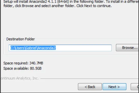
Choose the installation directory. You can leave the default or choose a different 3.
directory by clicking on Browse. We will go with the default and then click on
Next, as shown in Figure 3:
Algorithms and Tools
[ 13 ]
Make sure the options shown in Figure 4 are checked. This will ensure that 4.
Anaconda integrates seamlessly with the Python components, and that it will be the primary Python on your system:
Figure 4: Setting advanced options
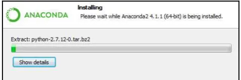
Wait while Anaconda is installed (refer to Figure 5): 5.
Algorithms and Tools
[ 14 ]
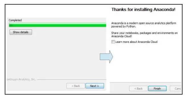
When the installation completes, click on Next and then on Finish, as you can see 6.
in Figure 6:
Figure 6: The installation has completed successfully
Congratulations! You have successfully installed Anaconda on your computer. To view the list of programs included with Anaconda, go to Start | All Programs | Anaconda2 (64-bit). Here's the list for your reference (the same applies if you're using other operating systems):
Anaconda Cloud: This is a collaboration and package-management tool for open
source and private projects. While public projects and notebooks are always free, private plans start at $7/month.
Anaconda Navigator: This is a desktop graphical user interface that allows us to
easily perform several operations without the need to use the command line.
Anaconda Prompt: This is a command prompt where you can issue Anaconda
and conda commands without having to change directories or add directories to
your PATH environment variable.
IPython: This is an interactive, robust, enhanced Python shell that includes extra
functionality.
Jupyter Notebook: As described on the project's website (http://jupyter.org
/), this is “a web application that allows you to create and share documents that contain live code, equations, visualizations and explanatory text.” You can think
Algorithms and Tools
[ 15 ]
Jupyter QTConsole: This is a widget that resembles a Python prompt but
includes several features that are only possible in a graphical user interface, such as graphics.
Spyder: This is a Python IDE for scientific programming. As such, it integrates
several Python libraries for this field, such as scikit-learn, pandas, and the well-known NumPy and matplotlib, to name a few.
Feel free to spend a few minutes becoming familiar with their interfaces. We will now explain the installation in Linux and will return to these programs later in this section.
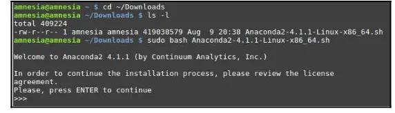
Installation in Linux Mint 18 (Mate desktop) 64-bit
To install Anaconda in Linux Mint 18 64-bit, you should have previously downloaded a Bash script named Anaconda2-x.y.z-Linux-x86_64.sh, where x.y.z represents the
current version of the program (4.1.1 at the time of writing). The most likely location where the script file will be found is Downloads, inside your home directory:
Browse to Downloads: 1.
cd ~/Downloads
List the files found therein to confirm: ls -l
To proceed with the installation, you will need to grant the script execute 2.
permissions (don't use sudo if you intend to save files in this directory using your
regular user account):
chmod +x Anaconda2-4.1.1-Linux-x86_64.sh
Then, source it from the current working directory:
sudo ./Anaconda2-4.1.1-Linux-x86_64.sh
Alternatively, you will need to run it directly with Bash (either method will work):
Algorithms and Tools
[ 16 ]
As indicated in Figure 7, you will need to press Enter to continue the installation: 3.
Figure 7: Starting the installation in Linux
You will then be able to view the license agreement. Use Enter to scroll down or q to close the document and type yes to indicate that you agree with the terms outlined in it, as shown in Figure 8:
Figure 8: Reviewing and accepting the license terms
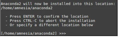
The default installation directory is ~/anaconda2. If you wish, you can choose a
4.
Algorithms and Tools
[ 17 ]
Figure 9: Choosing the installation directory
Near the end of the installation process, you will be asked whether you want the 5.
installer to include (prepend) the installation directory to your PATH
environment variable. If you choose the default (no), you will need to browse to the installation directory each time you want to execute one of the programs included with Anaconda. Otherwise (by choosing yes, as we did in this case), as shown in Figure 10, you will be able to run those programs directly when you launch your Linux terminal:
Figure 10: Adding the Anaconda installation directory to PATH
You can now view the list of installed applications in Linux in ~/anaconda2/bin. All of them consist of Python scripts that can be conveniently launched from the command line.
At this point, you should have the same set of tools installed on your computer regardless of your operating system choice. To wrap up with this section, launch Spyder:
In Windows, go to Start | All Programs | Anaconda2 (64-bit) | Spyder
Algorithms and Tools
[ 18 ]
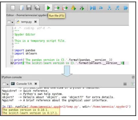
Once Spyder has opened, copy or type the following lines in the code area (left section), which should return the versions of scikit-learn and pandas currently installed in your environment:
import pandas import sklearn
print('The pandas version is {}.'.format(pandas.__version__))
print('The scikit-learn version is {}.'.format(sklearn.__version__))
Click on the Run file button or press F5. The output will be shown inside the IPython console in the bottom-right corner, as shown in Figure 11:
Figure 11: Viewing the currently installed versions of scikit-learn and pandas
When you open any of the utilities included with Anaconda, a command line (Linux) or command prompt (Windows) will be launched
Algorithms and Tools
[ 19 ]
Exploring a well-known dataset for machine
learning
Among other features, scikit-learn includes several out-of-the-box sample datasets. In the following example, we will import the Iris dataset directly using scikit-learn for simplicity. Additionally, The University of California at Irvine maintains a repository (http://archive .ics.uci.edu/ml/) with several collections of real-world datasets that can be used for free to analyze machine-learning algorithms.
The Iris dataset, one of the datasets included with scikit-learn, has long been used to demonstrate statistical techniques in machine learning. It consists of 50 samples from each of the three species of Iris (setosa,
virginica, and versicolor) where each sample contains four measurements, in centimeters: sepal length and width, and petal length and width. One can use these measurements to train a machine to predict the species of a new observation. You will probably be able to guess that we are looking at a supervised learning problem as it can help us predict the species of a given Iris, given the measurements of its sepal and petal.
The Iris dataset meets the requirements for working with scikit-learn:
The columns of the sample (also known as features) and the result we are trying to predict (also known as the response) must be separate objects. The features in this case are sepal length, sepal width, petal length, and petal width, whereas the response is 0, 1, and 2 (corresponding to the setosa, versicolor, and virginica species, respectively).
Both features and responses must be numeric (that's why each species is mapped to an integer, as explained in the previous requirement), must consist of a grid of values of the same type (known in the Python ecosystem as NumPy arrays), and must have specific, well-defined shapes (the size of the grid along rows and columns).
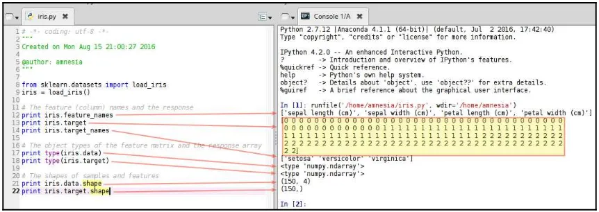
To demonstrate the requirements mentioned earlier, let's load the dataset into Spyder and print the following:
The feature (column) names and the response. Note how the actual species names are mapped to 0, 1, and 2.
Algorithms and Tools
[ 20 ]
To do that, copy the following code into the Spyder editor and save it as iris.py in your
home directory or Documents folder, and then press F5. The output will be shown in the IPython console on the right, as shown in Figure 12:
# coding: utf-8 """
Created on Mon Aug 15 21:00:27 2016 @author: amnesia
"""
from sklearn.datasets import load_iris iris = load_iris()
# The feature (column) names and the response print iris.feature_names
print iris.target print iris.target_names
# The object types of the feature matrix and the response array print type(iris.data)
print type(iris.target)
# The shapes of samples and features print iris.data.shape
Let's take a look at the result of the preceding code in Figure 12:
Algorithms and Tools
[ 21 ]
Training models and classification
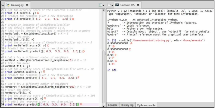
After loading the dataset and verifying that it meets the requirements for working with scikit-learn, it is time to use it to train a model and classify a new observation. We will actually use two models:
With LinearSVC (Support Vector Classifier), the dataset is categorized or divided by a hyperplane (https://en.wikipedia.org/wiki/Hyperplane) into classes. This hyperplane is often referred to as a Support Vector Machine, and represents the maximized division between the groups or classes. The response is given by the class where a new observation belongs.
Before we go ahead to train the model and obtain the predictions, let's consider a few conventions to write a new, improved version of the script we used before. This time we will name it training.py.
The sample data and the target (iris.data and iris.target in the preceding example) should be stored in variables X and y as they are a matrix and a vector,
respectively.
By default, scikit-learn assigns K = 5 for the K-nearest neighbors. If we want to
change this value, we can pass the n_neighbors=K argument to the instance of
the classifier (also known as the estimator).
With the K-nearest neighbors model, a prediction is made for a new observation by searching through the entire training dataset for the “K” most similar
observations (neighbors) based on the distance between them and the new sample. The response is then given by the class with the highest number of neighbor occurrences. In other words:
Given a dataset divided into classes A, B, and C, and a new observation, y, if we choose K = 3, the K-nearest neighbors model will search through the entire dataset for the three observations that are closest to y. If two of them belong to class A and the third one belongs to B, the algorithm will conclude that y belongs to A. The right number of neighbors to use as a parameter will depend on the number of samples and data sparsity:
# coding: utf-8 """
Created on Tue Aug 16 19:29:30 2016
Algorithms and Tools
from sklearn.neighbors import KNeighborsClassifier # Load the dataset
Algorithms and Tools
[ 23 ]
Let's take a look at the results in Figure 13 (match the letter in the script area with the corresponding letter in the console):
Figure 13: Predicting the class of a new observation using the LinearSVC and K-nearest neighbors algorithms
In the preceding figure, you can see how the prediction becomes less accurate when you increase the number of K in the K-nearest neighbor model. It does not make much sense to use 100 neighbors on a 150-observation dataset.
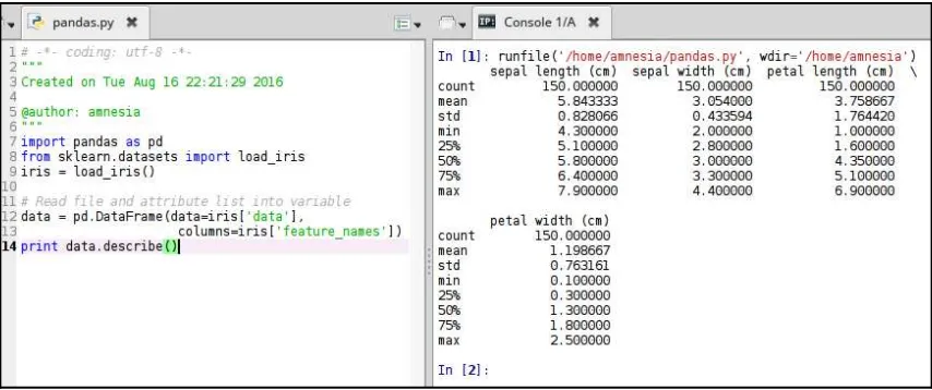
Finally, you might consider using pandas to describe a given dataset in statistical terms. Save the following code as pandas.py and press F5 to run it:
# coding: utf-8
"""
Created on Tue Aug 16 22:21:29 2016 @author: amnesia
"""
import pandas as pd
from sklearn.datasets import load_iris iris = load_iris()
# Read file and attribute list into variable data = pd.DataFrame(data=iris['data'],
Algorithms and Tools
[ 24 ]
In Figure 14, we will see the output of the preceding code. For each of the dataset features (sepal length/width, and petal length/width), several statistical measures are shown:
Figure 14
For example, we can see that the maximum sepal length is 7.9 cm, whereas the mean for petal width is 1.198667 cm. This goes to show that Pandas can do a great job at helping us summarize our dataset for statistical analysis.
All the code files shown in this book can be downloaded for free from the
3
Machine Learning and Big Data
In the previous two sections An Introduction to Machine Learning and Algorithms and Tools, we introduced the essential concepts and the types of machine learning. Also, we explained how to install Anaconda, a full-featured Python suite that includes all the tools necessary for this field of study.As the datasets used in the field of machine learning grows bigger and more complex, we enter the realm of big data–massive amounts of data, growing exponentially, and coming
from a variety of sources. This information needs to be analyzed and stored efficiently and rapidly in order to provide business value by enhancing insight and assisting in decision making and process automation. Additionally, size cannot by itself be used to identify big data. Complexity (we will see what this means in this section) is another important factor that must also be taken into account.
The challenges of big data
Unfortunately, big-data analysis cannot be accomplished using traditional processing methods. Some examples of big data sources are social media interactions, collection of geographical coordinates for Global Positioning Systems, sensor readings, and retail store transactions, to name a few. These examples give us a glimpse into what is known as the three Vs of big data:
Volume: Huge amounts of data that are being generated every moment
Variety: Different forms that data can come in–plain text, pictures, audio and
video, geospatial data, and so on
Machine Learning and Big Data
[ 26 ]
The wide variety of sources that a business or company can use to gather data for analysis results in large amounts of information–and it only keeps growing. This requires special
technologies for data storage and management that were not available or whose use was not widespread a decade ago.
Since big data is best handled through distributed computing instead of a single machine, we will only cover the fundamental concepts of this topic and its theoretical relationship with machine learning in the hope that it will serve as a solid starting point for a later study of the subject. You can rest assured that big data is a hot topic in modern technology, but don't just take our word for it–a simple Google search for big data salaries will
reveal that professionals in this area are being offered very lucrative compensation.
While machine learning will help us gain insight from data, big data will allow us to handle massive volumes of data. These disciplines can be used either together or separately.
The first V in big data – volume
When we talk about volume as one of the dimensions of big data, one of the challenges is the required physical space that is required to store it efficiently considering its size and projected growth. Another challenge is that we need to retrieve, move, and analyze this data efficiently to get the results when we need them. At this point, I am sure you will see that there are yet other challenges associated with the handling of high volumes of information–the availability and maintenance of high speed networks and sufficient
bandwidth, along with the related costs, are only two of them. For example, while a
traditional data analysis application can handle a certain amount of clients or retail stores, it may experience serious performance issues when scaled up 100x or 1000x. On the other hand, big data analysis–with proper tools and techniques–can lead to achieving a
cost-effective solution without damaging the performance.
Machine Learning and Big Data
[ 27 ]
As organizations and companies are able to boost the volume of information and utilize it as part of their analysis, their business insight is expanded accordingly: they are able to increase consumer satisfaction, improve travel safety, protect their reputation, and even save lives–wildfire and natural disasters prediction being some of the top examples in this
area.
The second V – variety
Variety does not only refer to the many sources where data comes from but also to the way it is represented (structural variety), the medium in which it gets delivered (medium
variety), and its availability over time.
As an example of structural variety, we can mention that the satellite image of a forming hurricane is different from tweets sent out by people who are observing it as it makes its way over an area. Medium variety refers to the medium in which the data gets delivered: an audio speech and the transcript may represent the same information but are delivered via different media. Finally, we must take into consideration that data may be available all the time, in real time (for example, a security camera), or only intermittently (when a satellite is over an area of interest).
Additionally, the study of data can't be restricted only to the analysis of structured data (traditional databases, tables, spreadsheets, and files), however, valuable these all-time resources can be. As we mentioned in the introduction, in the era of big data, lots of unstructured data (SMSes, images, audio files, and so on) is being generated, transmitted, and analyzed using special methods and tools (we will briefly describe one such tool toward the end of this section).
That said, it is no wonder that data scientists agree that variety actually means diversity and complexity.
The third V – velocity
When we consider Velocity as one of the dimensions of big data, we may think it only refers to the way it is transmitted from one point to another. However, as we indicated in the introduction, it means much more than that. It also implies the speed at which it is
Machine Learning and Big Data
[ 28 ]
Let's consider the following examples to illustrate the importance of velocity in big data analytics:
If you want to give your son or daughter a present for his or her birthday, would you consider what they wanted a year ago, or would you ask them what they would like today?
If you are considering moving to a new career, would you take into consideration the top careers from a decade ago or the ones that are most relevant today and are expected to experience a remarkable growth in the future?
These examples illustrate the importance of using the latest information available in order to make a better decision. In real life, being able to analyze data as it is being generated is what allows advertising companies to offer advertisements based on your recent past searches or purchases–almost in real time.
An application that illustrates the importance of velocity in big data is called sentiment analysis–the study of the public's feelings about products or events. In 2013, countries in the
European continent suffered what later became known as the horse-meat scandal.
According to Wikipedia (https://en.wikipedia.org/wiki/2013_horse_meat_scandal), foods advertised as containing beef were found to contain undeclared or improperly declared horse or pork meat–as much as 100% of the meat content in some cases. Although
horse meat is not harmful to health and is eaten in many countries, pork is a taboo food in the Muslim and Jewish communities.
Before the scandal hit the streets, Meltwater (a media intelligence firm) helped Danone, one of their customers, manage a potential reputation issue by alerting them about the breaking story that horse DNA had been found in meat products. Although Danone was confident that they didn't have this issue with their products, having this information a couple of hours in advance allowed them to run another thorough check. This, in turn, allowed them to reassure their customers that all their products were fine, resulting in an effective reputation-management operation.
Introducing a fourth V – veracity
Machine Learning and Big Data
[ 29 ]
In this context, quality actually means volatility (for how long will the current data be valid to be used for decision making?) and validity (it can contain noise, imprecisions, and biases). Additionally, it also depends on the reliability of the data source. Consider, for example, the fact that as the Internet of Things takes off, more and more sensors will enter the scene bringing some level of uncertainty as to the quality of the data being generated.
It is expected that, as new challenges emerge with big-data analysis, more Vs (or dimensions) will be added to the overall description of this field of study.
Why is big data so important?
The question inevitably arises, “Why is big data such a big deal in today's computing?” In
other words, what makes big data so valuable as to deserve million-dollar investments from big companies on a periodic basis? Let's consider the following real-life story to illustrate the answer.
In the early 2000s, a large retailer in the United States hired a statistician to analyze the shopping habits of its customers. In time, as his computers analyzed past sales associated with customer data and credit card information, he was able to assign a pregnancy prediction score and estimate due dates within a small window. Without going into the nitty-gritty of the story, it is enough to say that the retailer used this information to mail discount coupons to people buying a combination of several pregnancy and baby care products. Needless to say, this ended up increasing the retailer's revenue significantly. About one year later, after the retailer started using this model, this is what happened (taken from an article published by The New York Times on February of 2012):
A very angry parent visited one of the stores in Minneapolis and demanded to see the manager. He was clutching coupons that had been sent to his daughter, and he was angry, according to an employee who participated in the conversation. “My daughter got this in
the mail!” he said. “She's still in high school, and you're sending her coupons for baby
clothes and cribs? Are you trying to encourage her to get pregnant?”
The manager didn't have any idea what the man was talking about. He looked at the mailer. Sure enough, it was addressed to the man's daughter and contained advertisements for maternity clothing, nursery furniture, and pictures of smiling infants. The manager apologized and then called a few days later to apologize again.
On the phone, though, the father was somewhat abashed. “I had a talk with my daughter,”
he said. “It turns out there's been some activities in my house I haven't been completely
Machine Learning and Big Data
[ 30 ]
http://www.nytimes.com/2012/02/19/magazine/shopping-habits.html)
Moral of the story: big data means big money. Disclaimer: although I do not agree with the way personal data was collected and used in the example above, it serves our current purpose of demonstrating the use of big-data analysis.
MapReduce and Hadoop
After having described the dimensions of big data and illustrated why it is relevant for us today, we will introduce you to the tools that are being used to handle it.
During the early 2000s, Google and Yahoo were starting to experiment the challenges associated with the massive amounts of information they were handling. However, the challenge not only resided in the amounts but also in the complexity of the data (can you see any relationship with big data already?). As opposed to structured data, this
information could not be easily processed using traditional methods–if at all.
As a result of subsequent studies and joint effort, Hadoop was born as an efficient and cost-effective tool for reducing huge analytical problems to small tasks that can be executed in parallel on clusters made up of commodity (affordable) hardware. Hadoop can handle many data sources: sensor data, social network trends, regular table data, search engine queries and results, and geographical coordinates, which are only a few examples. In time, Hadoop grew to become a powerful and robust ecosystem that includes multiple tools to make the management of big data a walk in the park for data scientists. It is currently being maintained by the Apache Foundation at http://hadoop.apache.org/, with Yahoo being one of their main contributors. I highly encourage you to check out their website for more details on how to install and use Hadoop, since such topics are out of the scope of this nano guide.
4
SPAM Detection - a Real-World
Application of Machine Learning
In Section 2, Algorithms and Tools, we introduced the fundamental algorithms and tools used in the field of machine learning. Through the use of practical examples, we explained how to use the Anaconda suite and begin your study of this fascinating subject. In this section, we will discuss how to use these tools to perform SPAM e-mail detection, a real-world application of machine learning.SPAM definition
At one point or another, since the Internet became a huge communication channel, we have all suffered from what is known as SPAM. Also known as junk mail, SPAM can be defined as massive, undesired e-mail communications that are sent to large numbers of people without their authorization. While the contents vary from one case to another, it has been observed that the main topics of these mails are pharmacy products, gambling, weight loss, and phishing attempts (a scam by which a person is tricked into revealing personal or sensitive information that someone will later exploit illicitly).
It is important to note that SPAM is not only annoying but also expensive. Today, many people check their inboxes using a cell-phone data plan. Every e-mail requires an amount of data transfer, which the client must pay for. Additionally, SPAM costs money for Internet
Service Providers (ISPs) as it is transmitted through their servers and other network
SPAM Detection - a Real-World Application of Machine Learning
[ 32 ]
SPAM detection
The real-world application of machine learning that we will present in this chapter is in identifying e-mail messages that are SPAM and those that are not (commonly called HAM). It is important to note that the principles discussed in this section are also applicable to any data transmission that consists of a stream of characters. This includes not only e-mail messages, but also SMSes, tweets, and Facebook posts alike. We will base our experiments on a freely-available training dataset of more than 5,000 SMS messages that can be
downloaded from https://archive.ics.uci.edu/ml/machine-learning-databases /00228/smsspamcollection.zip.
The SPAM-detection example is a classification problem, a type of machine-learning problem that we discussed in Section 1, An Introduction to Machine Learning. In the present case, data is classified as SPAM or HAM based on the rules we will discuss in this section. By the way, the word HAM was coined in the early 2000s by people working on SpamBayes (http://spambayes.sourceforge.net/), the Python
probabilistic classifier, and has no actual meaning attached to it other than
“e-mail that is not SPAM.”
Before proceeding further, we will install TextBlob, a Python library for working with textual data. As it is only available for Mac OS X, we will install it manually:
pip install -U textblob
Depending on your system, you may need to install python-tools before executing the preceding command. If this utility is missing from your system, the installation will fail and alert you to do so. To install python-tools in Linux Mint for Python 2.7.x, run this
command:
aptitude install python-tools
For Python 3.x, run the following command:
aptitude install python3-tools
If you are using Windows 7 or higher, follow the instructions provided in the Package Index at https://pypi.python.org/pypi/setuptools.
SPAM Detection - a Real-World Application of Machine Learning
[ 33 ]
Training our machine-learning model
Once we have added TextBlob to the list of available Python libraries, we will work on setting up the training dataset and the SPAM detector file itself. To do so, follow these steps:
After downloading the ZIP file that contains the training dataset, unzip it to a 1.
location of your choice (but preferably inside your personal directory). Then, create a subdirectory named spamdetection to host the contents of the zip file and another one that we will add to process the training dataset.
Launch Spyder and create a new file inside spamdetection named detector.py.
2.
Next, add the following lines to that file:
# coding: utf-8
from sklearn.feature_extraction.text import CountVectorizer, TfidfTransformer
from sklearn.naive_bayes import MultinomialNB
Throughout this series of steps, you will be asked to add lines of code to
detector.py. If you forget to do so, you will not get the expected result.
Using detector.py, load the training dataset and print the total number of lines,
3.
each representing a record. Note that the rstrip() Python method is used to
strip whitespace characters from the end of each line. If you uncompressed the ZIP file in a directory other than spamdetection, you will need to specify the corresponding path as an argument to the following open() method:
# Load the training dataset 'SMSSpamCollection' into variable 'messages'
messages = [line.rstrip() for line in open('SMSSpamCollection')] # Print number of messages
SPAM Detection - a Real-World Application of Machine Learning
[ 34 ]
At this point, you should get the following message in the console if you execute
detector.py (refer to the following screenshot) by pressing F5:
Figure 1: Viewing the number of records in the training dataset
As you can see, the training dataset contains 5,574 records.
Inspect the messages by parsing the training dataset file (SMSSpamCollection)
4.
using pandas. The use of the head() method causes pandas to return only the
first five rows:
To preserve internal quotations in messages, use QUOTE_NONE. """
messages = pandas.read_csv('SMSSpamCollection', sep='\t', quoting=csv.QUOTE_NONE,
names=["class", "message"]) # Print first 5 records print messages.head()
Note that the first column has been labeled class, whereas the second column is
message, as we can see in the following screenshot. In class, we can see the
individual classification of each message as ham (good) or spam (bad):
SPAM Detection - a Real-World Application of Machine Learning
[ 35 ]
Using the samples in SMSSpamCollection, we will train a machine-learning
model to distinguish between spam and ham messages. This will allow us to later classify new messages under one of these two groups.
Use the groupby() and count() methods to group the records by class and then
5.
count the number in each one. Although this is not strictly required in our study, it is useful to learn more about the training dataset. As before, add the following line to detector.py, save the file, and press F5:
# Group by class and count
print messages.groupby('class').count()
The output should be similar to that shown in the following screenshot:
Figure 3: Grouping records by class
As you can see, there are 4,827 ham messages and 747 spam ones.
To split each message into a series of words, we will use the bag-of-words model. 6.
This is a common document classification technique where the occurrence and the frequency of each word is used to train a classifier. The presence (and especially the frequency) of words such as the ones mentioned under SPAM detection earlier is a pretty accurate indicator of spam.
The following function will allow us to split each message into a series of words:
# Split messages into individual words
SPAM Detection - a Real-World Application of Machine Learning
[ 36 ]
In Figure 4, we can see the result of the preceding function:
Figure 4 – The first five records split into their individual words
Normalize the words resulting from Step 6 into their base form and convert each 7.
message into a vector to train the model. In this step, words such as walking,
walked, walks, and walk are reduced into their lemma–walk. Thus, the presence of
any of those words will actually count toward the number of occurrences of walk:
# Convert each word into its base form def WordsIntoBaseForm(message):
message = unicode(message, 'utf8').lower() words = TextBlob(message).words
return [word.lemma for word in words] # Convert each message into a vector
trainingVector = CountVectorizer(analyzer=WordsIntoBaseForm) .fit(data['message'])
At this point, we can examine an arbitrary vector (message #10 in this example) and view the frequency of each individual word (see Figure 5):
# View occurrence of words in an arbitrary vector. Use 9 for vector #10.
SPAM Detection - a Real-World Application of Machine Learning
[ 37 ]
Figure 5 – Counting number of occurrences of each word in an arbitrary vector
Then inspect which words appear twice and three times using the feature number, a unique identification for each lemma. Using features numbers 3437 and 5192, we will view one of the words that is repeated twice and one that is repeated three times, as we can see in Figure 6. For easier comparison, we will also print the entire message (#10):
# Print message #10 for comparison print messages['message'][9] # Identify repeated words
print 'First word that appears twice:', trainingVector.get_feature_names()[3437] print 'Word that appears three times:', trainingVector.get_feature_names()[5192]
Figure 6 – Viewing repeated words in a message
Note how mobile, mobiles, and Mobile were considered as the same word, as were
SPAM Detection - a Real-World Application of Machine Learning
[ 38 ]
Take the term frequency (TF, the number of times a term occurs in a document) 8.
and inverse document frequency (IDF) of each word. The IDF diminishes the weight of a word that appears very frequently and increases the weight of words that do not occur often:
# Bag-of-words for the entire training dataset messagesBagOfWords = trainingVector.transform( messages['message'])
# Weight of words in the entire training dataset Term Frequency and Inverse Document Frequency
messagesTfidf = TfidfTransformer().fit(messagesBagOfWords) .transform(messagesBagOfWords)
Based on these preceding statistical values, we will be able to train our model using the Naive-Bayes algorithm. With scikit-learn, this is as easy as running
the following:
# Train the model
spamDetector = MultinomialNB().fit(messagesTfidf, data['class'].values)
Congratulations! You have trained your model to perform SPAM detection. Now we'll test it against new data.
The SPAM detector
The last challenge in this section consists of testing our model against new messages. To check whether a new message is spam or ham, pass it as a parameter to spamDetector, as
follows:
# Test message
example = ['England v Macedonia - dont miss the goals/team news. Txt ENGLAND to 99999']
# Result
SPAM Detection - a Real-World Application of Machine Learning
[ 39 ]
Figure 7 shows the result of running the preceding code, and a separate test with
Everything is OK, Mom as the message:
Figure 7 – Testing the SPAM-detector with two messages
As you can see, we have tested our model successfully with two test messages. Feel free to experiment with your own messages now.
All the code files shown in this book can be downloaded for free from the
machine-learning-packt repository under my GitHub account at https://github.com/gacanepa /machine-learning-packt.
Note that a full study of this subject, including the accuracy of the spam-detection results, is out of the scope of this nano book. You can find more information about the SPAM SMS training dataset at http://www.dt.fee.unicamp.br/~tiago/smsspamcollection/.
Summary
In this guide we introduced machine learning as a fascinating field of study and explained the different types through easy-to-understand, practical examples. Also, we learned how to install and use Anaconda, a full-feature Python-based suite for scientific data analysis. Using the tools for machine learning included in Anaconda, we reviewed a basic example (the Iris dataset) and a real-world application (SPAM detection) of classification–a core
SPAM Detection - a Real-World Application of Machine Learning
[ 40 ]
What to do next?
If you’re interested in Machine Learning, then you’ve come to the right place. We’ve got aTo learn more about Machine Learning and find out what you want to learn next, visit the Machine Learning technology page at https://www.packtpub.com/tech/Machine%20Learn ing.
If you have any feedback on this eBook, or are struggling with something we haven’t
covered, let us know at [email protected].