DOI: http://dx.doi.org/10.21609/jiki.v9i2.384
FEATURE SELECTION METHODS BASED ON MUTUAL INFORMATION FOR CLASSIFYING HETEROGENEOUS FEATURES
Ratri Enggar Pawening1, Tio Darmawan2, Rizqa Raaiqa Bintana2,3, Agus Zainal Arifin2 and Darlis Herumurti2
1Department of Informatics, STT Nurul Jadid Paiton, Jl. Pondok Pesantren Nurul Jadid Paiton, Probolinggo, 67291, Indonesia
2Department of Informatics Engineering, Faculty of Information Technology, Institut Teknologi Sepuluh Nopember (ITS), Kampus ITS Sukolilo, Surabaya, 60111, Indonesia
3Department of Informatics, Faculty of Science and Technology, UIN Sultan Syarif Kasim Riau, Jl. H.R Soebrantas, Pekanbaru, 28293, Indonesia
E-mail: [email protected], [email protected]2
Abstract
Datasets with heterogeneous features can affect feature selection results that are not appropriate
because it is difficult to evaluate heterogeneous features concurrently. Feature transformation (FT) is
another way to handle heterogeneous features subset selection. The results of transformation from non-numerical into numerical features may produce redundancy to the original numerical features. In this paper, we propose a method to select feature subset based on mutual information (MI) for classifying heterogeneous features. We use unsupervised feature transformation (UFT) methods and joint mutual information maximation (JMIM) methods. UFT methods is used to transform non-numerical features into non-numerical features. JMIM methods is used to select feature subset with a consideration of the class label. The transformed and the original features are combined entirely, then determine features subset by using JMIM methods, and classify them using support vector machine (SVM) algorithm. The classification accuracy are measured for any number of selected feature subset and compared between UFT-JMIM methods and Dummy-JMIM methods. The average classification accuracy for all experiments in this study that can be achieved by UFT-JMIM methods is about 84.47% and Dummy-JMIM methods is about 84.24%. This result shows that UFT-JMIM methods can minimize information loss between transformed and original features, and select feature subset to avoid redundant and irrelevant features.
Keywords: Feature selection, Heterogeneous features, Joint mutual information maximation, Support vector machine, Unsupervised feature transformation
Abstrak
Dataset dengan fitur heterogen dapat mempengaruhi hasil seleksi fitur yang tidak tepat karena sulit untuk mengevaluasi fitur heterogen secara bersamaan. Transformasi fitur adalah cara untuk mengatasi seleksi subset fitur yang heterogen. Hasil transformasi fitur non-numerik menjadi numerik mungkin menghasilkan redundansi terhadap fitur numerik original. Dalam tulisan ini, peneliti mengusulkan sebuah metode untuk seleksi subset fitur berdasarkan mutual information (MI) untuk klasifikasi fitur heterogen. Peneliti menggunakan metode unsupervised feature transformation (UFT) dan metode joint mutual information maximation (JMIM). Metode UFT digunakan untuk transformasi fitur non-numerik menjadi fitur non-numerik. Metode JMIM digunakan untuk seleksi subset fitur dengan pertimbangan label kelas. Fitur hasil transformasi dan fitur original disatukan seluruhnya, kemudian menentukan subset fitur menggunakan metode JMIM, dan melakukan klasifikasi terhadap subset fitur tersebut menggunakan algoritma support vector machine (SVM). Akurasi klasifikasi diukur untuk sejumlah subset fitur terpilih dan dibandingkan antara metode UFT-JMIM dan Dummy-JMIM. Akurasi klasifikasi rata-rata dari keseluruhan percobaan yang dapat dicapai oleh metode UFT-JMIM sekitar 84.47% dan metode Dummy-JMIM sekitar 84.24%. Hasil ini menunjukkan bahwa metode UFT-JMIM dapat meminimalkan informasi yang hilang diantara fitur hasil transformasi dan fitur original, dan menyeleksi subset fitur untuk menghindari fitur redundansi dan tidak relevan.
Kata Kunci: Fitur heterogen, Joint mutual information maximation, Seleksi fitur, Support vector machine, Unsupervised feature transformation
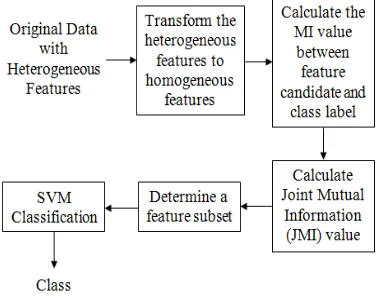
Figure 1. The proposed methods 1. Introduction
Data and features which have high-dimensional are the main problems in the classification of su-pervised and unsusu-pervised learning, which is be-coming even more important with the recent ex-plosion of the size of the available datasets both in terms of the number of data samples and the num-ber of features in each sample. The rapid training time and the enhancement of classification accu-racy can be obtained when dimension of data and features are decreased as low as possible.
Dimensionality reduction can be conducted using feature extraction and feature selection me-thods. Feature extraction methods transform the original features into a new feature which has lo-wer dimension. The common used methods are principal component analysis (PCA) [1-2] and li-near discriminant analysis (LDA) [3-4]. Feature selection methods is conducted by selecting some important features which minimises a cost func-tion.
Feature selection methods are divided into two categories in terms of evaluation strategy, in particular, classifier dependent and classifier inde -pendent. Classifier dependent is divided into two methods, wrapper and embedded methods. Wrap-per methods evaluate subsets of variables to detect the possible interactions between variables by me-asuring the prediction accuracy of a classifier. Wrapper methods had researched by [5-6]. They perform well because the selected subset is opti-mised for the classification algorithm. Wrapper methods may suffer from over-fitting to the learn-ing algorithm and has very expensive in computa-tional complexity, especially when handling extre-mely high-dimensional data. It means that each change of training models will decrease the func-tion of subsets.
The feature selection stage in the embedded methods is combined with the learning stage [6]. Embedded methods perform variable selection as part of the learning procedure and are usually spe-cific to given learning machines. These methods are less computational complexity and over-fitti-ng. However, they are very specific and difficult for generalisation.
Classifier independent can be called as filter methods. Filter methods assess the relevance of features by looking only at the intrinsic properties of the data. The advantages of filter methods are: they can scale of high-dimensional datasets, they are computationally simple and fast, and they are independent of the classification algorithm. The disadvantage of filter methods is that they ignore the interaction between the features and the classi-fier (the search in the feature subset space is sepa-rated from the search in the hypothesis space), and
most proposed techniques are univariate. Feature selection using filter methods is researched by [7]. These methods rank features according to their re-levance to the class label in the supervised learn-ing. The relevance score is calculated using mutu-al information (MI).
Information theory has been widely applied in filter methods, where information measures su-ch as mutual information are used as a measure of the features’s relevance and redundancy. MI can overcome problems of filter methods. Some me-thods which apply MI are MIFS [8], mRMR [9], NMIFS [10], and MIFS-ND [11]. These methods optimize the relationship between relevance and redundancy when selecting features. The proble-ms of these methods is the overestimation of the significance of the feature candidates. The method for selecting the most relevant features using joint mutual information (JMI) is proposed by [12]. Jo-int Mutual Information Maximation (JMIM) is the development of JMI that adds ma-ximum of the minimum method.
Datasets with heterogeneous features can af-fect feature selection results that are not appropri-ate because it is difficult to evaluappropri-ate heter ogene-ous features concurrently. Feature transformation (FT) is another way to handle heterogeneous fea-tures subset selection. FT methods unify the for-mat of datasets and enable traditional feature se-lection algorithms to handle heterogeneous data-sets. FT methods for heterogeneous features using unsupervised feature transformation (UFT) has proposed by [13]. The results of transformation from non-numerical into numerical features may produce redundancy to the original numerical fea-tures. The redundant features can be handled by selecting of the significant feature.
Secti-2, June 2016
Algorithm 1: UFT
Input: dataset D, which have heterogeneous feature fj,jє {1, ..., m}
Output: transformed dataset D' with pure numerical features generate numerical data and substitute the values equal to si in feature fj
10: end for 11: end if 12: end for on 3 describes the conducted experiments and
dis-cusses the results. Section 4 concludes this study.
2. Methods
General description of the research methods is sh-own in Figure 1. The stages of UFT-JMIM meth-ods in this study are transformation of heterogene-ous features, calculation of MI value between fea-ture candidate and class label, calculation of JMI value, determine a feature subset, and classificati-on by using SVM.
Transformation of heterogeneous features
In the transformation stage, we transform the da-tasets that have heterogeneous features to homo-geneous features. Feature transformation is con-ducted by using UFT methods.UFT is derived fr-om the analytical relationship between MI and en-tropy. The purpose of UFT is to find a numerical
X’ to substitute the ori-ginal non-numerical featu-re X, and X’ is constrai-ned by I(X’;X) = H(X). Th-is constraint makes the MI between the transform-ed X’ and the original X to be the same as the en-tropy of the original X.
This condition is critical because it ensures that the original feature information is preserved, when non-numerical features are transformed into numerical features. It is also worth noting that the transformation is independent of class label, so th-at the bias introduced by class label can be reduc-ed. After it is processed by UFT methods, the da-tasets’s format which have heterogeneous features can be combined to numerical features entirely. The solution for UFT methods is shown by equati-on(1) [13]. Based on equatiequati-on(1), UFT methods can be formalized as shown by Algorithm 1, whi-ch also details equation(1) together.
𝝁𝝁𝒊𝒊∗=�(𝒏𝒏 − 𝒊𝒊)− ∑𝒊𝒊𝒌𝒌=𝟏𝟏(𝒏𝒏 −
𝒌𝒌) 𝒑𝒑𝒌𝒌� ��𝟏𝟏 − ∑ 𝒑𝒑𝒊𝒊 𝒊𝒊𝟑𝟑� ∑ 𝒑𝒑� 𝒊𝒊≠𝒋𝒋 𝒊𝒊𝒑𝒑𝒋𝒋(𝒊𝒊 − 𝒋𝒋)𝟐𝟐, (1)
where 𝝈𝝈𝒊𝒊∗= 𝒑𝒑𝒊𝒊𝒊𝒊𝝐𝝐 {𝟏𝟏, … ,𝒏𝒏}
Calculation of MI value between feature candi-date and class label
MI is the amount of information that both variab-les share, and is defined as equation(2). Each fea-ture fi which is a member of F is calculated the
The value of p(ci) probability function is obtained by using equation(5). the already selected subset S if it satisfies equa-tion(6).
𝐈𝐈(𝐟𝐟𝐢𝐢,𝐒𝐒;𝐂𝐂) >𝐈𝐈(𝐟𝐟𝐣𝐣,𝐒𝐒;𝐂𝐂) (6)
Calculate JMI value
Let S = {f1, f2, …, fk}, JMI of fi and each feature in
S with C is calculated. The minimum value of this mutual information is selected based on the lowest amount of new information of feature fi that is added to subset. The feature that produces the ma-ximum value is the feature that adds mama-ximum in-formation to that shared bet-ween S and C, it mea-ns that the feature is most relevant to the class la-bel C in the context of the subset S according to equation(6).
Algorithm 2: Forward greedy search
1. (Initialisation) Set F← “initial set of n features”; S ← “empty set.”
2. (Computation of the MI with the output class) For
∀fiє F compute I(C; fi).
5. (Output) Output the set S with the selected features.
equation(8).
Determine a feature subset
The method uses the following iterative forward greedy search algorithm to find the relevant featu-re subset of size k within the feature space (Algo-rithm 2).
Classification process
At this stage, classification process is conducted to determine the class of the object. In this study, the cclassification uses support vector machine (SVM) multiclass One-Against-One (OAO) with polynomial kernel. Polynomial kernel function (K) is shown by equation(9):
𝑲𝑲(𝒎𝒎,𝒎𝒎𝒊𝒊) = [(𝒎𝒎.𝒎𝒎𝒊𝒊) +𝟏𝟏]𝒒𝒒 (9)
where xi is dimensional input (i = 1, 2, ..., l, l is the number of samples) belong to class 1 or ano-ther and q is power of polynomial kernel function.
Datasets
Datasets are used in this study from UCI Reposi-tory (table I). They are Acute Inflammations, Ad-ult, Australian Credit Approval, German Credit Data, and Hepatitis. Data type of Acute Inflamma-tions dataset is multivariate. The attribute types of this dataset are categorical and integer. This data-set contains 1 numerical feature and 5 non-nume-rical features. All of the non-numenon-nume-rical features
only have two probability values, yes or no value. This dataset has two classes of data, they are yes for the inflammation of urinary bladder and no for not.
Data type of Adult dataset is multivariate. This dataset contains 14 features that composed by categorical and integer values. The attribute ty-pes of this dataset are categorical and number. Ev-ery feature has different number of values. This dataset has two data classes.
Australian Credit Approval dataset has mul-tivariate data type. This dataset contains 14 featu-res that composed by categorical, number, and re-al vre-alues. There are 6 numericre-al features and 8 categoical features. This dataset has two data clas-ses. They are + (positive) class for approved credit and – (negative) class for rejected credit.
Data type of German Credit Data dataset is multivariate. This dataset contains 20 features that composed by categorical and number. There are 7 numerical features and 13 categorical features. This dataset has two classes of data, they are 1 as good credit consumer and 2 as bad credit consu-mer.
Data type of Hepatitis dataset is multivariate. The dataset contains 20 features that composed by categorical, number, and real values. There are 6 numerical features and 13 categorical features. This dataset has two classes of data, they are 1 for die and 2 for live.
3. Results and Analysis
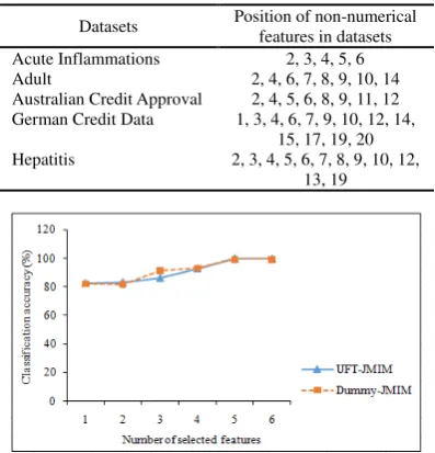
To validate the results of proposed methods, five datasets from UCI Repository are used in the ex-periment (Table 1). In the datasets used, the type of non-numerical features is categorical data whi-ch is nominal and ordinal data type. The number of non-numerical features in each dataset is diffe-rent (Table 2).
Scenario of testing is conducted by transfor-ming non-numerical features using UFT methods and dummy variable. The transformation using dummy variable is conducted by changing the da-ta to the numbers manually, for example feature of sex which has male and female data is changed by numeral 1 (for male) and 2 (for female).
It means Dummy-JMIM has lower comple-xity than UFT-JMIM but we do not know it is go-od for changing the categorical value manually or no. The transformed and the original features are combined entirely, then determine features subset by using JMIM methods, and classify them using SVM algorithm. The classification accuracy are measured for any number of selected feature sub-set and compared between UFT-JMIM methods and Dummy-JMIM methods.
whi-2, June 2016
TABLE 1
DESCRIPTION OF REAL-WORLD DATASETS
1 2 3 4 5 6
Acute Inflammations
120 2 1 5 6
Adult 1992 2 6 8 14
Australian Credit Approval
690 2 6 8 14
German Credit Data
1000 2 7 13 20
Hepatitis 80 2 6 13 19
Titles of column heads:
1: Datasets; 2: Instances; 3: Classes; 4: Numerical features 5: Non-numerical features; 6: Features
TABLE 2
NON-NUMERICAL FEATURES IN DATASETS
Datasets Position of non-numerical features in datasets Acute Inflammations 2, 3, 4, 5, 6
Adult 2, 4, 6, 7, 8, 9, 10, 14
Australian Credit Approval 2, 4, 5, 6, 8, 9, 11, 12 German Credit Data 1, 3, 4, 6, 7, 9, 10, 12, 14,
15, 17, 19, 20 Hepatitis 2, 3, 4, 5, 6, 7, 8, 9, 10, 12,
13, 19
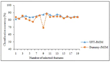
Figure. 4. The classification accuracy that is achieved by the Acute Inflammations dataset
Figure. 3. The classification accuracy that is achieved by the Adult dataset
Figure. 2. The classification accuracy that is achieved by the Australian Credit Approval dataset
ch is created to represent an attribute with two or more different categories or levels. We use dum-my variable as another way for the trans-forma-tion of features by using defined variable. Dummy variable is used as a reference to ensure that the results of transformation from non-numerical into numerical features by using UFT methods does not have significant difference to the results of transformation of features using defined variable. So that, indicating that the original feature infor-mation is not lost.
Figures 2-6 show the classification accuracy of the five datasets. The classification accuracy is computed for the whole size of the selected subset (from 1 feature up to 20 features). Thus, all featu-res of each dataset in this experiment was selected for each testing of k value (number of selected fe-atures). As shown in Figure 2, it illustrates the ex-periment with the acute inflammations dataset. UFT-JMIM achieves the highest average accuracy (100%) with 5 and 6 selected features, which is higher than the accuracy of Dummy-JMIM with 5 features (99.5%) and 6 features (99.4%).
In Figure. 3 which illustates the accuracy of the adult dataset, UFT-JMIM cannot achieve the highest classification accuracy. It can only achieve the 74.9% with 12 selected features. Meanwhile, Dummy-JMIM can achieve classification accura-cy 77.1% with 14 features. Figure 4 shows the re-sults for australian credit approval dataset. UFT-JMIM can achieve the highest classification result (85.83%) with 11 selected features. Dummy-JMIM can achieve the closest classification accu-racy (85.80%) with 14 features.
The classification accuracy of UFT-JMIM for german credit data dataset is shown by Figure 5. It achieves 72.3% (15 selected features). Whe-reas, the classification accuracy produced by Du-mmy-JMIM can only achieve 70.6% as the best result with 1 selected feature. Figure 6 shows the UFT-JMIM performance for the hepatitis dataset which achieves the highest classification accuracy (89.3%) with 10 selected features. Meanwhile, Dummy-JMIM can only achieve 88.2% with 10 selected features.
ori-Figure. 6. The classification accuracy that is achieved by the German Credit Data dataset
Figure. 5. The classification accuracy that is achieved by the Hepatitis dataset
ginal features to preserve the original feature in-formation.
In addition, MI applied in JMIM methods is used to measure of relevant and redundant featu-res when select feature subset. It studies relevancy and redundancy, and takes into consideration the class label when calculating MI. In this methods, the candidate feature that maximises the cumula-tive summation of joint mutual information with features of the selected subset is chosen and added to the subset. JMIM methods employs joint mutu-al information and the ‘maximum of the minim-um’ approach, which should choose the most rele-vant features. The features are selected by JMIM according to criterion as equation(7). In JMIM methods, the iterative forward greedy search al-gorithm is used to find the best combination of k
features within subset. It causes the performance of finding to feature subset to be suboptimal be-cause of high computation.
4. Conclusion
Feature selection based on MI using trans-formed features can reduce the redundancy of the selected feature subset, so that it can improve the accuracy of classification. The average classification accu-racy for all experiments in this study that can be achieved by UFT-JMIM methods is about 84.47% and Dummy-JMIM methods is about 84.24%. Th-is result shows that UFT-JMIM methods can mi-nimize information loss between transformed and original features, and select feature subset to avo-id redundant and irrelevant features.
For future work, further improvement can be made by studying to determine the best size k to find the relevant feature subset from heterogene-ous features automatically in which it may make computation to be low.
References
[1] Bajwa, I., Naweed, M., Asif, M., & Hyder, S., “Feature based image classification by using principal component analysis,” ICGST International Journal on Graphics Vision and Image Processing, vol. 9, pp. 11–17. 2009.
[2] Turk, M., & Pentland, A., “Eigenfaces for re-cognition,” Journal of Cognitive Neuro-sci-ence, vol. 3, pp. 72–86. 1991.
[3] Tang, E. K., Suganthana, P. N., Yao, X., & Qina, A. K., “Linear dimensionality reducti-on using relevance weighted LDA,” Pattern Recognition, vol. 38, pp. 485–493. 2005. [4] Yu, H., & Yang, J., “A direct LDA algorithm
for high-dimensional data with application to face recognition,” Pattern Recognition, vol. 34, pp. 2067–2070. 2001.
[5] Bennasar, M., Hicks, Y., & Setchi, Rossitza, “Feature selection using Joint Mutual Infor-mation Maximisation,” Expert Systems With Applications, vol. 42, pp. 8520-8532. 2015. [6] Guyon, I., Gunn, S., Nikravesh, M., &
Za-deh, L.A., Feature extraction foundations and applications, Springer Studies infuzzi--ness and soft computing, New York/Berlin, Heidelberg, 2006.
[7] Saeys, Y., Inza, I., & Larrañaga, P., “A revi-ew of feature selection techniques in bioin-formatics,” Bioinformatics Advance Access, vol. 23, pp. 2507-2517. 2007.
[8] Battiti, R., “Using mutual information for se-lecting features in supervised neural net lear-ning,” IEEE Transactions on Neural Net-works, vol. 5, pp. 537–550. 1994.
[9] Peng, H., Long, F., & Ding, C., “Feature sel-ection based on mutual information: criteria of max-dependency, max-relevance, and min -redundancy,” IEEE Transactions on Pattern Analysis and Machine Intelligence, vol. 27, pp. 1226–1238. 2005.
2, June 2016
[11] Hoque, N., Bhattacharyya, D. K., & Kalita, J. K., “MIFS-ND: a mutual information ba-sed feature selection method,” Expert Sys-tems with Applications, vol. 41, pp. 6371– 6385. 2014.
[12] Yang, H., & Moody, J., “Feature selection based on joint mutual information” In Pro-ceedings of international ICSC sympo-sium
on advances in intelligent data analysis, pp. 22–25, 1999.