C H A P T E R
2
Algorithm Analysis
An algorithmis a clearly specified set of simple instructions to be followed to solve a problem. Once an algorithm is given for a problem and decided (somehow) to be correct, an important step is to determine how much in the way of resources, such as time or space, the algorithm will require. An algorithm that solves a problem but requires a year is hardly of any use. Likewise, an algorithm that requires hundreds of gigabytes of main memory is not (currently) useful on most machines.
In this chapter, we shall discuss
rHow to estimate the time required for a program.
rHow to reduce the running time of a program from days or years to fractions of a second.
rThe results of careless use of recursion.
rVery efficient algorithms to raise a number to a power and to compute the greatest common divisor of two numbers.
2.1 Mathematical Background
The analysis required to estimate the resource use of an algorithm is generally a theoretical issue, and therefore a formal framework is required. We begin with some mathematical definitions.
Throughout the book we will use the following four definitions:
Definition 2.1.
T(N) =O(f(N)) if there are positiveconstants candn0 such thatT(N)≤ cf(N) when
N≥n0.
Definition 2.2.
T(N) = (g(N)) if there are positiveconstants candn0such thatT(N)≥cg(N) when
N≥n0.
Definition 2.3.
T(N)=!(h(N)) if and only ifT(N)=O(h(N)) andT(N)= (h(N)).
Definition 2.4.
T(N)=o(p(N)) if for all positive constantscthere exists ann0such thatT(N)<cp(N) whenN>n0. Less formally,T(N)=o(p(N)) ifT(N)=O(p(N)) andT(N)#=!(p(N)).
The idea of these definitions is to establish a relative order among functions. Given two functions, there are usually points where one function is smaller than the other function, so it does not make sense to claim, for instance,f(N) < g(N). Thus, we compare their relative rates of growth.When we apply this to the analysis of algorithms, we shall see why this is the important measure.
Although 1,000Nis larger thanN2for small values ofN,N2grows at a faster rate, and thusN2will eventually be the larger function. The turning point isN=1,000 in this case. The first definition says that eventually there is some pointn0past whichc·f(N) is always at least as large asT(N), so that if constant factors are ignored, f(N) is at least as big as T(N). In our case, we haveT(N)=1,000N,f(N)=N2,n0=1,000, andc=1. We could also usen0=10 andc=100. Thus, we can say that 1,000N=O(N2) (orderN-squared). This notation is known asBig-Oh notation. Frequently, instead of saying “order . . . ,” one says “Big-Oh . . . .”
If we use the traditional inequality operators to compare growth rates, then the first definition says that the growth rate of T(N) is less than or equal to (≤) that of f(N). The second definition, T(N) = (g(N)) (pronounced “omega”), says that the growth rate ofT(N) is greater than or equal to (≥) that of g(N). The third definition, T(N) = !(h(N)) (pronounced “theta”), says that the growth rate of T(N) equals (=) the growth rate ofh(N). The last definition, T(N) = o(p(N)) (pronounced “little-oh”), says that the growth rate of T(N) is less than (<) the growth rate of p(N). This is different from Big-Oh, because Big-Oh allows the possibility that the growth rates are the same.
To prove that some function T(N) = O(f(N)), we usually do not apply these defini-tions formally but instead use a repertoire of known results. In general, this means that a proof (or determination that the assumption is incorrect) is a very simple calculation and should not involve calculus, except in extraordinary circumstances (not likely to occur in an algorithm analysis).
When we say thatT(N)=O(f(N)), we are guaranteeing that the functionT(N) grows at a rate no faster thanf(N); thusf(N) is anupper boundonT(N). Since this implies that f(N)= (T(N)), we say thatT(N) is alower boundonf(N).
As an example, N3 grows faster thanN2, so we can say thatN2 = O(N3) orN3 =
(N2).f(N)= N2 andg(N)= 2N2 grow at the same rate, so bothf(N) = O(g(N)) and
2.1 Mathematical Background 31
Function Name
c Constant
logN Logarithmic
log2N Log-squared
N Linear
NlogN
N2 Quadratic
N3 Cubic
2N Exponential
Figure 2.1 Typical growth rates
The important things to know are
Rule 1.
IfT1(N)=O(f(N)) andT2(N)=O(g(N)), then
(a)T1(N)+T2(N)=O(f(N)+g(N)) (intuitively and less formally it is
O(max(f(N),g(N))) ),
(b)T1(N)∗T2(N)=O(f(N)∗g(N)).
Rule 2.
IfT(N) is a polynomial of degreek, thenT(N)=!(Nk).
Rule 3.
logkN=O(N) for any constantk. This tells us that logarithms grow very slowly.
This information is sufficient to arrange most of the common functions by growth rate (see Figure 2.1).
Several points are in order. First, it is very bad style to include constants or low-order terms inside a Big-Oh. Do not sayT(N)=O(2N2) orT(N)=O(N2+N). In both cases, the correct form isT(N) =O(N2). This means that in any analysis that will require a Big-Oh answer, all sorts of shortcuts are possible. Lower-order terms can generally be ignored, and constants can be thrown away. Considerably less precision is required in these cases.
Second, we can always determine the relative growth rates of two functionsf(N) and g(N) by computing limN→∞f(N)/g(N), using L’Hôpital’s rule if necessary.1The limit can
have four possible values:
rThe limit is 0: This means thatf(N)=o(g(N)). rThe limit isc#=0: This means thatf(N)=!(g(N)).
1L’Hôpital’s rule states that if lim
N→∞f(N) = ∞ and limN→∞g(N) = ∞, then limN→∞f(N)/g(N) =
rThe limit is∞: This means thatg(N)=o(f(N)).
rThe limit does not exist: There is no relation (this will not happen in our context).
Using this method almost always amounts to overkill. Usually the relation between f(N) and g(N) can be derived by simple algebra. For instance, if f(N) = NlogN and g(N) = N1.5, then to decide which of f(N) and g(N) grows faster, one really needs to determine which of logNandN0.5grows faster. This is like determining which of log2N orNgrows faster. This is a simple problem, because it is already known thatNgrows faster than any power of a log. Thus,g(N) grows faster thanf(N).
One stylistic note: It is bad to sayf(N)≤O(g(N)), because the inequality is implied by the definition. It is wrong to writef(N)≥O(g(N)), which does not make sense.
As an example of the typical kinds of analysis that are performed, consider the problem of downloading a file over the Internet. Suppose there is an initial 3-sec delay (to set up a connection), after which the download proceeds at 1.5 M(bytes)/sec. Then it follows that if the file isNmegabytes, the time to download is described by the formulaT(N)=
N/1.5+3. This is alinear function. Notice that the time to download a 1,500M file (1,003 sec) is approximately (but not exactly) twice the time to download a 750M file (503 sec). This is typical of a linear function. Notice, also, that if the speed of the connection doubles, both times decrease, but the 1,500M file still takes approximately twice the time to download as a 750M file. This is the typical characteristic of linear-time algorithms, and it is why we writeT(N) = O(N), ignoring constant factors. (Although using Big-Theta would be more precise, Big-Oh answers are typically given.)
Observe, too, that this behavior is not true of all algorithms. For the first selection algorithm described in Section 1.1, the running time is controlled by the time it takes to perform a sort. For a simple sorting algorithm, such as the suggested bubble sort, when the amount of input doubles, the running time increases by a factor of four for large amounts of input. This is because those algorithms are not linear. Instead, as we will see when we discuss sorting, trivial sorting algorithms areO(N2), or quadratic.
2.2 Model
In order to analyze algorithms in a formal framework, we need a model of computation. Our model is basically a normal computer, in which instructions are executed sequentially. Our model has the standard repertoire of simple instructions, such as addition, multipli-cation, comparison, and assignment, but, unlike the case with real computers, it takes exactly one time unit to do anything (simple). To be reasonable, we will assume that, like a modern computer, our model has fixed-size (say, 32-bit) integers and that there are no fancy operations, such as matrix inversion or sorting, that clearly cannot be done in one time unit. We also assume infinite memory.
2.3 What to Analyze 33
2.3 What to Analyze
The most important resource to analyze is generally the running time. Several factors affect the running time of a program. Some, such as the compiler and computer used, are obviously beyond the scope of any theoretical model, so, although they are important, we cannot deal with them here. The other main factors are the algorithm used and the input to the algorithm.
Typically, the size of the input is the main consideration. We define two functions, Tavg(N) andTworst(N), as the average and worst-case running time, respectively, used by an algorithm on input of sizeN. Clearly,Tavg(N) ≤ Tworst(N). If there is more than one input, these functions may have more than one argument.
Occasionally the best-case performance of an algorithm is analyzed. However, this is often of little interest, because it does not represent typical behavior. Average-case perfor-mance often reflects typical behavior, while worst-case perforperfor-mance represents a guarantee for performance on any possible input. Notice, also, that, although in this chapter we ana-lyze Java code, these bounds are really bounds for the algorithms rather than programs. Programs are an implementation of the algorithm in a particular programming language, and almost always the details of the programming language do not affect a Big-Oh answer. If a program is running much more slowly than the algorithm analysis suggests, there may be an implementation inefficiency. This is more common in languages (like C++) where arrays can be inadvertently copied in their entirety, instead of passed with references. However, this can occur in Java, too. Thus in future chapters we will analyze the algorithms rather than the programs.
Generally, the quantity required is the worst-case time, unless otherwise specified. One reason for this is that it provides a bound for all input, including particularly bad input, which an average-case analysis does not provide. The other reason is that average-case bounds are usually much more difficult to compute. In some instances, the definition of “average” can affect the result. (For instance, what is average input for the following problem?)
As an example, in the next section, we shall consider the following problem:
Maximum Subsequence Sum Problem.
Given (possibly negative) integersA1,A2,. . .,AN, find the maximum value ofjk=iAk. (For convenience, the maximum subsequence sum is 0 if all the integers are negative.) Example:
For input−2, 11,−4, 13,−5,−2, the answer is 20 (A2throughA4).
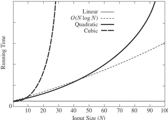
This problem is interesting mainly because there are so many algorithms to solve it, and the performance of these algorithms varies drastically. We will discuss four algo-rithms to solve this problem. The running time on some computer (the exact computer is unimportant) for these algorithms is given in Figure 2.2.
Algorithm Time
Input 1 2 3 4
Size O(N3) O(N2) O(NlogN) O(N)
N=100 0.000159 0.000006 0.000005 0.000002
N=1,000 0.095857 0.000371 0.000060 0.000022
N=10,000 86.67 0.033322 0.000619 0.000222
N=100,000 NA 3.33 0.006700 0.002205
N=1,000,000 NA NA 0.074870 0.022711
Figure 2.2 Running times of several algorithms for maximum subsequence sum (in seconds)
programs are now too slow, because they used poor algorithms. For large amounts of input, algorithm 4 is clearly the best choice (although algorithm 3 is still usable).
Second, the times given do not include the time required to read the input. For algo-rithm 4, the time merely to read in the input from a disk is likely to be an order of magnitude larger than the time required to solve the problem. This is typical of many efficient algorithms. Reading the data is generally the bottleneck; once the data are read, the problem can be solved quickly. For inefficient algorithms this is not true, and significant computer resources must be used. Thus it is important that, whenever possible, algorithms be efficient enough not to be the bottleneck of a problem.
Notice that algorithm 4, which is linear, exhibits the nice behavior that as the prob-lem size increases by a factor of ten, the running time also increases by a factor of ten.
0
Running
T
ime
10 20 30 40 50 60 70 80 90 100 Input Size (N)
Linear
O(N log N)
Quadratic Cubic
2.4 Running Time Calculations 35
0 0
Running
T
ime
1000 2000 3000 4000 5000 6000 7000 8000 9000 10000 Input Size (N)
Linear
O(N log N)
Quadratic Cubic
Figure 2.4 Plot (Nvs. time) of various algorithms
Algorithm 2, which is quadratic, does not have this behavior; a tenfold increase in input size yields roughly a hundredfold (102) increase in running time. And algorithm 1, which is cubic, yields a thousandfold (103) increase in running time. We would expect algorithm 1 to take nearly 9,000 seconds (or two and half hours) to complete forN = 100,000. Similarly, we would expect algorithm 2 to take roughly 333 seconds to complete for N = 1,000,000. However, it is possible that Algorithm 2 could take somewhat longer to complete due to the fact thatN =1,000,000 could also yield slower memory accesses thanN=100,000 on modern computers, depending on the size of the memory cache.
Figure 2.3 shows the growth rates of the running times of the four algorithms. Even though this graph encompasses only values of N ranging from 10 to 100, the relative growth rates are still evident. Although the graph for theO(NlogN) algorithm seems linear, it is easy to verify that it is not by using a straight-edge (or piece of paper). Although the graph for theO(N) algorithm seems constant, this is only because for small values ofN, the constant term is larger than the linear term. Figure 2.4 shows the performance for larger values. It dramatically illustrates how useless inefficient algorithms are for even moderately large amounts of input.
2.4 Running Time Calculations
Generally, there are several algorithmic ideas, and we would like to eliminate the bad ones early, so an analysis is usually required. Furthermore, the ability to do an analysis usually provides insight into designing efficient algorithms. The analysis also generally pinpoints the bottlenecks, which are worth coding carefully.
To simplify the analysis, we will adopt the convention that there are no particular units of time. Thus, we throw away leading constants. We will also throw away low-order terms, so what we are essentially doing is computing a Big-Oh running time. Since Big-Oh is an upper bound, we must be careful never to underestimate the running time of the program. In effect, the answer provided is a guarantee that the program will terminate within a certain time period. The program may stop earlier than this, but never later.
2.4.1 A Simple Example
Here is a simple program fragment to calculateN i=1i3:
public static int sum( int n ) {
int partialSum;
1 partialSum = 0;
2 for( int i = 1; i <= n; i++ )
3 partialSum += i * i * i; 4 return partialSum;
}
The analysis of this fragment is simple. The declarations count for no time. Lines 1 and 4 count for one unit each. Line 3 counts for four units per time executed (two multiplica-tions, one addition, and one assignment) and is executedNtimes, for a total of 4Nunits. Line 2 has the hidden costs of initializingi, testingi≤ N, and incrementingi. The total cost of all these is 1 to initialize,N+1 for all the tests, andNfor all the increments, which is 2N+2. We ignore the costs of calling the method and returning, for a total of 6N+4. Thus, we say that this method isO(N).
If we had to perform all this work every time we needed to analyze a program, the task would quickly become infeasible. Fortunately, since we are giving the answer in terms of Big-Oh, there are lots of shortcuts that can be taken without affecting the final answer. For instance, line 3 is obviously anO(1) statement (per execution), so it is silly to count precisely whether it is two, three, or four units; it does not matter. Line 1 is obviously insignificant compared with theforloop, so it is silly to waste time here. This leads to several general rules.
2.4.2 General Rules
Rule 1—forloops.
2.4 Running Time Calculations 37
Rule 2—Nested loops.
Analyze these inside out. The total running time of a statement inside a group of nested loops is the running time of the statement multiplied by the product of the sizes of all the loops.
As an example, the following program fragment isO(N2):
for( i = 0; i < n; i++ ) for( j = 0; j < n; j++ )
k++;
Rule 3—Consecutive Statements.
These just add (which means that the maximum is the one that counts; see rule 1(a) on page 31).
As an example, the following program fragment, which hasO(N) work followed byO(N2) work, is alsoO(N2):
for( i = 0; i < n; i++ ) a[ i ] = 0;
for( i = 0; i < n; i++ ) for( j = 0; j < n; j++ )
a[ i ] += a[ j ] + i + j;
Rule 4—if/else. For the fragment
if( condition ) S1
else S2
the running time of anif/elsestatement is never more than the running time of the test plus the larger of the running times of S1 and S2.
Clearly, this can be an overestimate in some cases, but it is never an underestimate. Other rules are obvious, but a basic strategy of analyzing from the inside (or deepest part) out works. If there are method calls, these must be analyzed first. If there are recursive methods, there are several options. If the recursion is really just a thinly veiledforloop, the analysis is usually trivial. For instance, the following method is really just a simple loop and isO(N):
public static long factorial( int n ) {
if( n <= 1 ) return 1; else
This example is really a poor use of recursion. When recursion is properly used, it is difficult to convert the recursion into a simple loop structure. In this case, the analysis will involve a recurrence relation that needs to be solved. To see what might happen, consider the following program, which turns out to be a horrible use of recursion:
public static long fib( int n ) {
1 if( n <= 1 )
2 return 1; else
3 return fib( n - 1 ) + fib( n - 2 ); }
At first glance, this seems like a very clever use of recursion. However, if the program is coded up and run for values ofN around 40, it becomes apparent that this program is terribly inefficient. The analysis is fairly simple. LetT(N) be the running time for the method callfib(n). IfN = 0 orN = 1, then the running time is some constant value, which is the time to do the test at line 1 and return. We can say thatT(0) = T(1) = 1 because constants do not matter. The running time for other values ofNis then measured relative to the running time of the base case. ForN>2, the time to execute the method is the constant work at line 1 plus the work at line 3. Line 3 consists of an addition and two method calls. Since the method calls are not simple operations, they must be analyzed by themselves. The first method call isfib(n - 1)and hence, by the definition ofT, requires T(N−1) units of time. A similar argument shows that the second method call requires T(N−2) units of time. The total time required is thenT(N−1)+T(N−2)+2, where the 2 accounts for the work at line 1 plus the addition at line 3. Thus, forN≥2, we have the following formula for the running time offib(n):
T(N)=T(N−1)+T(N−2)+2
Sincefib(N)=fib(N−1)+fib(N−2), it is easy to show by induction thatT(N)≥fib(N). In Section 1.2.5, we showed thatfib(N) < (5/3)N. A similar calculation shows that (for N>4)fib(N)≥(3/2)N, and so the running time of this program growsexponentially.This is about as bad as possible. By keeping a simple array and using aforloop, the running time can be reduced substantially.
2.4 Running Time Calculations 39
2.4.3 Solutions for the Maximum Subsequence
Sum Problem
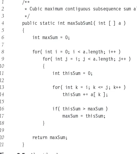
We will now present four algorithms to solve the maximum subsequence sum prob-lem posed earlier. The first algorithm, which merely exhaustively tries all possibilities, is depicted in Figure 2.5. The indices in theforloop reflect the fact that in Java, arrays begin at 0, instead of 1. Also, the algorithm does not compute the actual subsequences; additional code is required to do this.
Convince yourself that this algorithm works (this should not take much convincing). The running time isO(N3) and is entirely due to lines 13 and 14, which consist of anO(1) statement buried inside three nestedforloops. The loop at line 8 is of sizeN.
The second loop has sizeN−iwhich could be small but could also be of sizeN. We must assume the worst, with the knowledge that this could make the final bound a bit high. The third loop has sizej−i+1, which, again, we must assume is of sizeN. The total isO(1·N·N·N) =O(N3). Line 6 takes onlyO(1) total, and lines 16 and 17 take only O(N2) total, since they are easy expressions inside only two loops.
It turns out that a more precise analysis, taking into account the actual size of these loops, shows that the answer is!(N3) and that our estimate above was a factor of 6 too high (which is all right, because constants do not matter). This is generally true in these kinds of problems. The precise analysis is obtained from the sumN−1
i=0
2 * Cubic maximum contiguous subsequence sum algorithm.
3 */
4 public static int maxSubSum1( int [ ] a )
which tells how many times line 14 is executed. The sum can be evaluated inside out, using formulas from Section 1.2.3. In particular, we will use the formulas for the sum of the firstNintegers and firstNsquares. First we have
j
This sum is computed by observing that it is just the sum of the firstN−iintegers. To complete the calculation, we evaluate
We can avoid the cubic running time by removing aforloop. This is not always pos-sible, but in this case there are an awful lot of unnecessary computations present in the algorithm. The inefficiency that the improved algorithm corrects can be seen by noticing thatj
k=iAk=Aj+ j−1
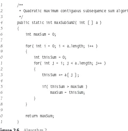
k=iAk, so the computation at lines 13 and 14 in algorithm 1 is unduly expensive. Figure 2.6 shows an improved algorithm. Algorithm 2 is clearlyO(N2); the analysis is even simpler than before.
There is a recursive and relatively complicated O(NlogN) solution to this problem, which we now describe. If there didn’t happen to be anO(N) (linear) solution, this would be an excellent example of the power of recursion. The algorithm uses a “divide-and-conquer” strategy. The idea is to split the problem into two roughly equal subproblems, which are then solved recursively. This is the “divide” part. The “conquer” stage consists of patching together the two solutions of the subproblems, and possibly doing a small amount of additional work, to arrive at a solution for the whole problem.
2.4 Running Time Calculations 41
1 /**
2 * Quadratic maximum contiguous subsequence sum algorithm.
3 */
4 public static int maxSubSum2( int [ ] a )
5 {
6 int maxSum = 0;
7
8 for( int i = 0; i < a.length; i++ )
9 {
10 int thisSum = 0;
11 for( int j = i; j < a.length; j++ )
12 {
13 thisSum += a[ j ];
14
15 if( thisSum > maxSum )
16 maxSum = thisSum;
17 }
18 }
19
20 return maxSum;
21 }
Figure 2.6 Algorithm 2
in the first half, and the largest sum in the second half that includes the first element in the second half. These two sums can then be added together. As an example, consider the following input:
First Half Second Half
4 −3 5 −2 −1 2 6 −2
The maximum subsequence sum for the first half is 6 (elementsA1throughA3) and for the second half is 8 (elementsA6throughA7).
The maximum sum in the first half that includes the last element in the first half is 4 (elementsA1throughA4), and the maximum sum in the second half that includes the first element in the second half is 7 (elementsA5 throughA7). Thus, the maximum sum that spans both halves and goes through the middle is 4+7=11 (elementsA1throughA7).
We see, then, that among the three ways to form a large maximum subsequence, for our example, the best way is to include elements from both halves. Thus, the answer is 11. Figure 2.7 shows an implementation of this strategy.
1 /**
2 * Recursive maximum contiguous subsequence sum algorithm.
3 * Finds maximum sum in subarray spanning a[left..right].
4 * Does not attempt to maintain actual best sequence.
5 */
6 private static int maxSumRec( int [ ] a, int left, int right )
7 {
8 if( left == right ) // Base case
9 if( a[ left ] > 0 )
10 return a[ left ];
11 else
12 return 0;
13
14 int center = ( left + right ) / 2;
15 int maxLeftSum = maxSumRec( a, left, center );
16 int maxRightSum = maxSumRec( a, center + 1, right );
17
18 int maxLeftBorderSum = 0, leftBorderSum = 0;
19 for( int i = center; i >= left; i-- )
20 {
21 leftBorderSum += a[ i ];
22 if( leftBorderSum > maxLeftBorderSum )
23 maxLeftBorderSum = leftBorderSum;
24 }
25
26 int maxRightBorderSum = 0, rightBorderSum = 0;
27 for( int i = center + 1; i <= right; i++ )
28 {
29 rightBorderSum += a[ i ];
30 if( rightBorderSum > maxRightBorderSum )
31 maxRightBorderSum = rightBorderSum;
32 }
33
34 return max3( maxLeftSum, maxRightSum,
35 maxLeftBorderSum + maxRightBorderSum );
36 }
37
38 /**
39 * Driver for divide-and-conquer maximum contiguous
40 * subsequence sum algorithm.
41 */
42 public static int maxSubSum3( int [ ] a )
43 {
44 return maxSumRec( a, 0, a.length - 1 );
45 }
2.4 Running Time Calculations 43
delimit the portion of the array that is operated upon. A one-line driver program sets this up by passing the borders 0 andN−1 along with the array.
Lines 8 to 12 handle the base case. Ifleft == right, there is one element, and it is the maximum subsequence if the element is nonnegative. The caseleft > rightis not possible unlessNis negative (although minor perturbations in the code could mess this up). Lines 15 and 16 perform the two recursive calls. We can see that the recursive calls are always on a smaller problem than the original, although minor perturbations in the code could destroy this property. Lines 18 to 24 and 26 to 32 calculate the two maximum sums that touch the center divider. The sum of these two values is the maximum sum that spans both halves. The routinemax3(not shown) returns the largest of the three possibilities.
Algorithm 3 clearly requires more effort to code than either of the two previous algo-rithms. However, shorter code does not always mean better code. As we have seen in the earlier table showing the running times of the algorithms, this algorithm is considerably faster than the other two for all but the smallest of input sizes.
The running time is analyzed in much the same way as for the program that computes the Fibonacci numbers. LetT(N) be the time it takes to solve a maximum subsequence sum problem of sizeN. IfN =1, then the program takes some constant amount of time to execute lines 8 to 12, which we shall call one unit. Thus,T(1) = 1. Otherwise, the program must perform two recursive calls, the twoforloops between lines 19 and 32, and some small amount of bookkeeping, such as lines 14 and 18. The twoforloops combine to touch every element in the subarray, and there is constant work inside the loops, so the time expended in lines 19 to 32 isO(N). The code in lines 8 to 14, 18, 26, and 34 is all a constant amount of work and can thus be ignored compared withO(N). The remainder of the work is performed in lines 15 and 16. These lines solve two subsequence problems of sizeN/2 (assumingNis even). Thus, these lines takeT(N/2) units of time each, for a total of 2T(N/2). The total time for the algorithm then is 2T(N/2)+O(N). This gives the equations
T(1)=1
T(N)=2T(N/2)+O(N)
To simplify the calculations, we can replace theO(N) term in the equation above with N; sinceT(N) will be expressed in Big-Oh notation anyway, this will not affect the answer. In Chapter 7, we shall see how to solve this equation rigorously. For now, if T(N) =
2T(N/2)+N, andT(1)=1, thenT(2)=4=2∗2,T(4)=12=4∗3,T(8)=32=8∗4, andT(16)=80=16∗5. The pattern that is evident, and can be derived, is that ifN=2k, thenT(N)=N∗(k+1)=NlogN+N=O(NlogN).
This analysis assumesNis even, since otherwiseN/2 is not defined. By the recursive nature of the analysis, it is really valid only whenN is a power of 2, since otherwise we eventually get a subproblem that is not an even size, and the equation is invalid. When Nis not a power of 2, a somewhat more complicated analysis is required, but the Big-Oh result remains unchanged.
1 /**
2 * Linear-time maximum contiguous subsequence sum algorithm.
3 */
4 public static int maxSubSum4( int [ ] a )
5 {
6 int maxSum = 0, thisSum = 0;
7
8 for( int j = 0; j < a.length; j++ )
9 {
10 thisSum += a[ j ];
11
12 if( thisSum > maxSum )
13 maxSum = thisSum;
14 else if( thisSum < 0 )
15 thisSum = 0;
16 }
17
18 return maxSum;
19 }
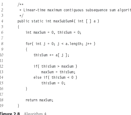
Figure 2.8 Algorithm 4
It should be clear why the time bound is correct, but it takes a little thought to see why the algorithm actually works. To sketch the logic, note that, like algorithms 1 and 2, jis representing the end of the current sequence, whileiis representing the start of the current sequence. It happens that the use ofican be optimized out of the program if we do not need to know where the actual best subsequence is, so in designing the algorithm, let’s pretend thatiis needed, and that we are trying to improve algorithm 2. One observation is that ifa[i]is negative, then it cannot possibly represent the start of the optimal sequence, since any subsequence that begins by includinga[i] would be improved by beginning witha[i+1]. Similarly, any negative subsequence cannot possibly be a prefix of the optimal subsequence (same logic). If, in the inner loop, we detect that the subsequence froma[i] toa[j]is negative, then we can advancei. The crucial observation is that not only can we advanceitoi+1, but we can also actually advance it all the way toj+1. To see this, letpbe any index betweeni+1andj. Any subsequence that starts at indexpis not larger than the corresponding subsequence that starts at indexiand includes the subsequence froma[i] toa[p-1], since the latter subsequence is not negative (jis the first index that causes the subsequence starting at indexito become negative). Thus advancingitoj+1is risk free: we cannot miss an optimal solution.
2.4 Running Time Calculations 45
test much of the code logic by comparing it with an inefficient (but easily implemented) brute-force algorithm using small input sizes.
An extra advantage of this algorithm is that it makes only one pass through the data, and once a[i] is read and processed, it does not need to be remembered. Thus, if the array is on a disk or is being transmitted over the Internet, it can be read sequentially, and there is no need to store any part of it in main memory. Furthermore, at any point in time, the algorithm can correctly give an answer to the subsequence problem for the data it has already read (the other algorithms do not share this property). Algorithms that can do this are calledonline algorithms. An online algorithm that requires only constant space and runs in linear time is just about as good as possible.
2.4.4 Logarithms in the Running Time
The most confusing aspect of analyzing algorithms probably centers around the logarithm. We have already seen that some divide-and-conquer algorithms will run inO(NlogN) time. Besides divide-and-conquer algorithms, the most frequent appearance of logarithms centers around the following general rule:An algorithm is O(logN)if it takes constant(O(1)) time to cut the problem size by a fraction (which is usually12).On the other hand, if constant time is required to merely reduce the problem by a constantamount(such as to make the problem smaller by 1), then the algorithm isO(N).
It should be obvious that only special kinds of problems can beO(logN). For instance, if the input is a list ofNnumbers, an algorithm must take (N) merely to read the input in. Thus, when we talk aboutO(logN) algorithms for these kinds of problems, we usually presume that the input is preread. We provide three examples of logarithmic behavior.
Binary Search
The first example is usually referred to as binary search.
Binary Search.
Given an integerXand integersA0,A1,. . .,AN−1, which are presorted and already in memory, findisuch thatAi=X, or returni= −1 ifXis not in the input.
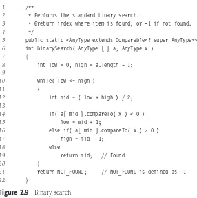
The obvious solution consists of scanning through the list from left to right and runs in linear time. However, this algorithm does not take advantage of the fact that the list is sorted and is thus not likely to be best. A better strategy is to check ifX is the middle element. If so, the answer is at hand. IfXis smaller than the middle element, we can apply the same strategy to the sorted subarray to the left of the middle element; likewise, ifXis larger than the middle element, we look to the right half. (There is also the case of when to stop.) Figure 2.9 shows the code for binary search (the answer ismid). As usual, the code reflects Java’s convention that arrays begin with index 0.
1 /**
2 * Performs the standard binary search.
3 * @return index where item is found, or -1 if not found.
4 */
5 public static <AnyType extends Comparable<? super AnyType>>
6 int binarySearch( AnyType [ ] a, AnyType x )
7 {
8 int low = 0, high = a.length - 1;
9
10 while( low <= high )
11 {
12 int mid = ( low + high ) / 2;
13
14 if( a[ mid ].compareTo( x ) < 0 )
15 low = mid + 1;
16 else if( a[ mid ].compareTo( x ) > 0 )
17 high = mid - 1;
18 else
19 return mid; // Found
20 }
21 return NOT_FOUND; // NOT_FOUND is defined as -1
22 }
Figure 2.9 Binary search
the maximum values ofhigh - lowafter each iteration are 64, 32, 16, 8, 4, 2, 1, 0,−1.) Thus, the running time isO(logN). Equivalently, we could write a recursive formula for the running time, but this kind of brute-force approach is usually unnecessary when you understand what is really going on and why.
Binary search can be viewed as our first data structure implementation. It supports the containsoperation inO(logN) time, but all other operations (in particularinsert) require O(N) time. In applications where the data are static (that is, insertions and deletions are not allowed), this could be very useful. The input would then need to be sorted once, but afterward accesses would be fast. An example is a program that needs to maintain information about the periodic table of elements (which arises in chemistry and physics). This table is relatively stable, as new elements are added infrequently. The element names could be kept sorted. Since there are only about 118 elements, at most eight accesses would be required to find an element. Performing a sequential search would require many more accesses.
Euclid’s Algorithm
2.4 Running Time Calculations 47
1 public static long gcd( long m, long n )
2 {
3 while( n != 0 )
4 {
5 long rem = m % n;
6 m = n;
7 n = rem;
8 }
9 return m;
10 }
Figure 2.10 Euclid’s algorithm
The algorithm works by continually computing remainders until 0 is reached. The last nonzero remainder is the answer. Thus, ifM=1,989 andN=1,590, then the sequence of remainders is 399, 393, 6, 3, 0. Therefore,gcd(1989, 1590)=3. As the example shows, this is a fast algorithm.
As before, estimating the entire running time of the algorithm depends on determining how long the sequence of remainders is. Although logNseems like a good answer, it is not at all obvious that the value of the remainder has to decrease by a constant factor, since we see that the remainder went from 399 to only 393 in the example. Indeed, the remainder does notdecrease by a constant factor in one iteration. However, we can prove that after two iterations, the remainder is at most half of its original value. This would show that the number of iterations is at most 2 logN = O(logN) and establish the running time. This proof is easy, so we include it here. It follows directly from the following theorem.
Theorem 2.1.
IfM>N, thenMmodN<M/2.
Proof.
There are two cases. If N ≤ M/2, then since the remainder is smaller than N, the theorem is true for this case. The other case isN>M/2. But thenNgoes intoMonce with a remainderM−N<M/2, proving the theorem.
One might wonder if this is the best bound possible, since 2 logNis about 20 for our example, and only seven operations were performed. It turns out that the constant can be improved slightly, to roughly 1.44 logN, in the worst case (which is achievable ifMandN are consecutive Fibonacci numbers). The average-case performance of Euclid’s algorithm requires pages and pages of highly sophisticated mathematical analysis, and it turns out that the average number of iterations is about (12 ln 2 lnN)/π2+1.47.
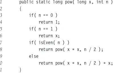
Exponentiation
1 public static long pow( long x, int n )
2 {
3 if( n == 0 )
4 return 1;
5 if( n == 1 )
6 return x;
7 if( isEven( n ) )
8 return pow( x * x, n / 2 );
9 else
10 return pow( x * x, n / 2 ) * x;
11 }
Figure 2.11 Efficient exponentiation
(or a compiler that can simulate this). We will count the number of multiplications as the measurement of running time.
The obvious algorithm to computeXNusesN−1 multiplications. A recursive algorithm can do better.N ≤ 1 is the base case of the recursion. Otherwise, ifNis even, we have XN=XN/2·XN/2, and ifNis odd,XN=X(N−1)/2·X(N−1)/2·X.
For instance, to compute X62, the algorithm does the following calculations, which involve only nine multiplications:
X3=(X2)X,X7=(X3)2X,X15=(X7)2X,X31=(X15)2X,X62=(X31)2
The number of multiplications required is clearly at most 2 logN, because at most two multiplications (ifNis odd) are required to halve the problem. Again, a recurrence formula can be written and solved. Simple intuition obviates the need for a brute-force approach.
Figure 2.11 implements this idea.2 It is sometimes interesting to see how much the code can be tweaked without affecting correctness. In Figure 2.11, lines 5 to 6 are actually unnecessary, because ifN is 1, then line 10 does the right thing. Line 10 can also be rewritten as
10 return pow( x, n - 1 ) * x;
without affecting the correctness of the program. Indeed, the program will still run in O(logN), because the sequence of multiplications is the same as before. However, all of the following alternatives for line 8 are bad, even though they look correct:
8a return pow( pow( x, 2 ), n / 2 );
8b return pow( pow( x, n / 2 ), 2 );
8c return pow( x, n / 2 ) * pow( x, n / 2 );
2Java provides aBigIntegerclass that can be used to manipulate arbitrarily large integers. Translating
Summary 49
Both lines 8a and 8b are incorrect because whenNis 2, one of the recursive calls topow has 2 as the second argument. Thus no progress is made, and an infinite loop results (in an eventual abnormal termination).
Using line 8c affects the efficiency, because there are now two recursive calls of sizeN/2 instead of only one. An analysis will show that the running time is no longerO(logN). We leave it as an exercise to the reader to determine the new running time.
2.4.5 A Grain of Salt
Sometimes the analysis is shown empirically to be an overestimate. If this is the case, then either the analysis needs to be tightened (usually by a clever observation), or it may be that theaverage running time is significantly less than the worst-case running time and no improvement in the bound is possible. For many complicated algorithms the worst-case bound is achievable by some bad input but is usually an overestimate in practice. Unfortunately, for most of these problems, an average-case analysis is extremely complex (in many cases still unsolved), and a worst-case bound, even though overly pessimistic, is the best analytical result known.
Summary
This chapter gives some hints on how to analyze the complexity of programs. Unfortunately, it is not a complete guide. Simple programs usually have simple analyses, but this is not always the case. As an example, later in the text we shall see a sorting algo-rithm (Shellsort, Chapter 7) and an algoalgo-rithm for maintaining disjoint sets (Chapter 8), each of which requires about 20 lines of code. The analysis of Shellsort is still not com-plete, and the disjoint set algorithm has an analysis that is extremely difficult and requires pages and pages of intricate calculations. Most of the analyses that we will encounter here will be simple and involve counting through loops.
An interesting kind of analysis, which we have not touched upon, is lower-bound analysis. We will see an example of this in Chapter 7, where it is proved that any algorithm that sorts by using only comparisons requires (NlogN) comparisons in the worst case. Lower-bound proofs are generally the most difficult, because they apply not to an algorithm but to a class of algorithms that solve a problem.