Short Papers
Dynamic Point-to-Point Trajectory Planning of a Two-DOF Cable-Suspended Parallel Robot
Cl´ement Gosselin and Simon Foucault
Abstract—This paper presents two trajectory-planning approaches for the point-to-point motion of planar two-degree-of-freedom (dof) cable-suspended parallel mechanisms. The proposed techniques can be used to plan trajectories that extend beyond the static workspace of the mechanism. Trajectories are specified as a list of target points that must be reached in sequence, with a zero velocity at each of the target points. In the first techn-nique, polynomial trajectories are designed to connect the target points, while the second approach uses trigonometric functions. Both techniques ensure continuity of the accelerations. Based on the dynamic model of the robot, algebraic inequalities are obtained that represent the constraints on cable tensions. These inequalities are used to determine the feasibility of the planned trajectories. Polynomial trajectories must be discretized in or-der to verify feasibility, while trajectories that are based on trigonometric functions can be verified globally, based on a set of simple algebraic equa-tions. Example trajectories are given in order to illustrate the approach. An experimental validation is also presented using a two-dof prototype, and two video extensions are provided to demonstrate the results.
Index Terms—Cable-driven robots, cable-suspended robots, dynamics, parallel robots, path planning for manipulators.
I. INTRODUCTION
Cable-suspended parallel robots have parallel cable-driven mecha-nisms which consist of a set of fixed actuators each driving a winch that controls a cable that is attached to a common moving platform. Cable-suspended robots rely on gravity to maintain their cables in tension. As opposed to other fully constrained cable-driven parallel robots such as those presented in [1] and [2] (and many others), cable-suspended robots are not necessarily redundantly actuated; they generally include as many actuators as degrees of freedom.
Cable-suspended parallel robots have been proposed in the liter-ature as potential candidates for applications that require very large workspaces or as mechanisms that can provide effective payload to mass ratios. One of the first cable-suspended mechanisms that was built is the Robocrane [3], which was developed by the National In-stitute of Standards and Technology two decades ago for crane-type operations. Other cable-suspended mechanisms have also been studied and prototypes were built to validate their performance (see, for in-stance, [4] and [5]). A commercially available cable-suspended system was also developed [6] for the video capture of sporting events.
Manuscript received March 13, 2013; revised August 28, 2013; accepted November 20, 2013. Date of publication January 31, 2014; date of current ver-sion June 3, 2014. This paper was recommended for publication by Associate Editor V. Krovi and Editor W. K. Chung upon evaluation of the reviewers’ comments. This work was supported by the Natural Sciences and Engineering Research Council of Canada and by the Canada Research Chair Program.
The authors are with the Department of Mechanical Engineering, Univer-sit´e Laval, Qu´ebec, QC G1V 0A6, Canada (e-mail: [email protected]; [email protected]).
This paper has supplementary downloadable material available at http://ieeexplore.ieee.org.
Color versions of one or more of the figures in this paper are available online at http://ieeexplore.ieee.org.
Digital Object Identifier 10.1109/TRO.2013.2292451
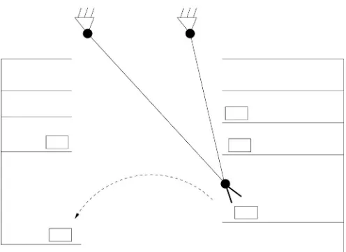
Fig. 1. Example application of a planar two-dof cable-suspended robot that requires trajectories extending beyond the static workspace.
In most cases found in the literature or implemented in practice, cable-suspended robots are assumed to work in static or quasi-static conditions. Therefore, most of the work reported in the literature does not address the dynamics of cable-suspended robots and uses tech-niques that are based on static equilibrium in order to solve control and design problems. For example, under the quasi-static assumption, the workspace of a cable-suspended robot is limited to configurations (poses) for which static equilibrium can be reached while maintaining all cables under tension. Such a workspace can never extend beyond the footprint of the robot. Techniques to determine the static workspace of cable-suspended robots were proposed in the literature, for instance, in [7].
More recently, cable-suspended robots have been envisioned as dy-namically controllable devices. In [8]–[11], dydy-namically controlled (pendulum-like) cable-suspended robots were proposed. The dynamic trajectory planning of cable-suspended robots opens new possibilities. Most importantly, their workspace can then extend beyond the static workspace and the notion of dynamic workspace [12] arises. The dy-namic workspace is defined as the set of poses that the platform can reach with at least one kinematic state (position, velocity and acceler-ation). In other words, the platform can reach points beyond the static workspace with a controlled kinematic state (e.g., a zero velocity but nonzero acceleration). Potential applications for pendulum-like cable-suspended robots that can move beyond their static workspace include the storage and retrieval of objects in a warehouse, as illustrated in Fig. 1. In such an application, restrictions on the footprint of the ca-ble attachment points due to potential interferences between the caca-bles and the environment may necessitate trajectories that include points outside the static workspace. Other potential applications include en-tertainment systems and stage performance mechanisms. For instance, moving objects over the audience with a cable-suspended mechanism for which the footprint of the attachment points is limited to the stage itself or moving acrobats along trajectories more complex than those possible with classical trapezes.
The pendulum-like robots proposed in [8]–[11] are underactuated, i.e., they include fewer actuators than degrees of freedom. Therefore, the trajectory of their end effector cannot be controlled exactly since the
dynamics of the uncontrolled degree(s) of freedom must be accounted for. The techniques proposed in the latter references focus on the deter-mination of actuator inputs that are capable of producing point-to-point motion between prescribed poses. Such techniques require the online numerical integration of the differential equation associated with the pendulum-like dynamics.
In [13], a planar two-dof robot suspended on two cables was consid-ered. As opposed to the mechanisms studied in the [8]–[11], the latter mechanism is not underactuated. Therefore, if the cables remain under tension, the dynamics of the robot are determined, and no numerical in-tegration is required in order to plan trajectories. Additionally, the realm of feasible trajectories is significantly augmented because the uncon-strained dof is eliminated. In [13], periodic trajectories were defined in the parametric form, and conditions on the parameters were obtained to ensure feasibility. It was shown that simple conditions on the trajectory parameters can be obtained which allow the planning of straight line or circular periodic trajectories. This technique was extended to three-dof spatial robots in [14]. However, in practice cable-suspended robots that are used beyond their static workspace will most likely be required to perform point-to-point motion, which is not compatible with periodic trajectories.
In this paper, the point-to-point dynamic trajectory planning of a planar two-dof cable-suspended robot is addressed. The trajectories are specified as a list of target points that must be reached in sequence, with a zero velocity at each of the target points. Two mathematical techniques are proposed to plan the motion. In the first technnique, polynomial trajectories are designed to connect the target points. Con-tinuity up to the acceleration level is ensured by a proper choice of trajectory parameters, and the travel time between consecutive points is determined in order to maximize the likelihood of obtaining fea-sible trajectories, i.e., trajectories that maintain tension in the cables. Finally, the trajectories are discretized in order to verify their feasibil-ity. In the second approach, trigonometric functions are used to design the trajectory segments between consecutive points. Continuity up to the acceleration level is ensured by adjusting the trajectory parame-ters. Because of the known bounds on the trigonometric functions, the feasibility of the trajectories can be determined using simple algebraic relationships, and no discretization is required.
This paper is arranged as follows. Section II presents the kinematic and dynamic modeling. In Section III, some results on the trajectory planning of simple periodic motions are briefly recalled. Section IV introduces the two novel trajectory-planning techniques developed here to plan point-to-point motion of the cable-suspended mechanism. Section V provides example trajectories and results obtained with the two types of trajectory-planning techniques developed in this paper. Finally, video extensions demonstrating the implementation on a pro-totype are included in order to illustrate the results.
II. KINEMATIC ANDDYNAMICMODELING
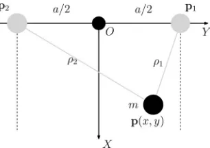
The planar two-dof cable-suspended robot addressed in this study is represented schematically in Fig. 2. It consists of two actuated spools mounted on a fixed structure which are used to control the extension of two cables. The cables are attached to a common end effector which is considered as a point mass. By controlling the extension of the two cables, the position of the point mass can be controlled. The robot has two actuators and two dofs and is therefore fully actuated. However, because the cables can only work in tension (they cannot push), con-straints must be imposed on the Cartesian trajectory prescribed at the end effector. The static workspace of the robot, i.e., the portion of the Cartesian space in which the end effector can be brought to rest, is lim-ited by vertical lines passing through the cable attachment points on the
Fig. 2. Planar two-dof cable-suspended robot.
structure. One of the objectives of this study is to produce trajectories that connect consecutive prescribed points that may be located beyond the boundaries of the static workspace.
Referring to the two-dof cable-suspended robot of Fig. 2, a fixed reference frame is defined on the base of the robot, whose origin is located on the line that connects the spool output points and at an equal distance from these points. TheY-axis is defined along this line which is assumed to be horizontal and theX-axis is vertical, pointing downward. The distance between the spool output points is noteda. The (constant) position vectors of these points can then be written as
p1 = [0, a/2]T andp
2 = [0,−a/2]T. The position vector of the end-effector point massm is notedp= [x, y]T. The cable lengths, i.e., the joint coordinates, are respectively notedρ1 andρ2. The inverse kinematic model of the robot is written as
ρi=
(p−pi)T(p−pi), i= 1,2. (1)
The dynamic model of the robot is obtained by considering the force balance on the point mass end effector, namely
2
whereFiis the tension in cablei,iis a unit vector along the direction of theX-axis, andgis the gravitational acceleration.
Equation (2) can be considered as a system of two linear equations in two unknowns (tensionsF1andF2) that can be explicitly solved for
F1 andF2 as
In order to ensure that the cables remain taut, it must be guaranteed that the tensionsF1 andF2remain positive at all times. Using (3), and assuming thatx >0(i.e., the end effector remains below the spools), the following conditions are obtained [13]:
(g−x¨)(y+a/2) +xy >¨ 0 (5)
(g−x¨)(y−a/2) +xy <¨ 0. (6)
III. TRAJECTORYPLANNING FORPERIODICSTEADY-STATEMOTION The dynamic model developed above was used in [13] to design feasible periodic trajectories that extend beyond the static workspace for the cable-suspended two-dof robot. Vertical, horizontal, and circular trajectories were constructed in the latter reference, and it was shown that special frequencies exist that can be used to produce arbitrarily large amplitudes of motion. The case of periodic horizontal motion is now briefly recalled for quick reference.
Consider a periodic horizontal motion along a direction parallel to theY-axis. The trajectory can be described mathematically as
x=x0, y=rsin(ωt), x0 >0 (7)
˙
x= 0, y˙=rωcos(ωt) (8)
¨
x= 0, y¨=−rω2sin(ωt) (9)
wherex0 is the distance between the (horizontal)Y-axis and the hori-zontal trajectory,ris one half of the total horizontal range of motion,ω
is the frequency of the periodic motion, andtis the time. Substituting the above parametric equations into inequalities (5) and (6) leads to
ga/2 + (gr−x0rω2) sin(ωt)>0 (10)
−ga/2 + (gr−x0rω2) sin(ωt)<0. (11)
Given the bounds on the sine function, the above conditions are satisfied throughout the trajectory if the following single condition is satisfied:
When inequality (12) is satisfied, the horizontal trajectory can be per-formed while maintaining both cables in tension. Since condition (12) involves the position of the trajectoryx0 as well as its amplituderand frequencyω, these parameters can be adjusted to produce globally fea-sible trajectories. One notable case occurs if the following frequency is used:
ωn =
g x0
. (13)
Referring to inequality (12), it is readily observed that, using this spe-cial frequency, arbitrary amplitudes of motionrcan theoretically be produced. This frequency,ωn, can be thought of as a kind ofnatural
frequencyfor the robot that performs horizontal oscillations. It is also remarkable that this frequency corresponds to the natural frequency of a single cable pendulum of lengthx0.
IV. POINT-TO-POINTDYNAMICTRAJECTORYPLANNING Although periodic trajectories are very useful to provide insight into the fundamental properties of the mechanism and although they can be used in some specific applications, most practical situations require that the robot be moved from one target point to another, in sequence. For instance, the robot can be required to reach a series of positions, some or all of which could be located outside of the static workspace. In applications for which the footprint of the attachment points of the robot is constrained while the workspace must be maximized, allowing the robot to reach target points that are located outside of the static workspace with a zero instantaneous velocity becomes an important requirement.
A. Polynomial Formulation
Assume that a series of prescribed points, whose position is given by vectorpi = [xi, yi]T withi∈[0,1, . . . , n], must be reached in se-quence. A polynomial formulation is used in order to devise trajectory
segments that connect two consecutive points while matching initial and final conditions on position, velocity, and acceleration. The pro-posed polynomial trajectories are inspired from [15]. Indeed, since six end-point conditions are prescribed (initial and final position, velocity and accleration), a fifth-degree polynomial is used. One such polyno-mial is used for each of the Cartesian dof of the mechanism.
For the trajectory segment connecting pointito point(i+ 1), one can design the polynomial trajectory associated with the motion in the
x-direction (vertical motion) as
x(t) =xi+ (xi+ 1−xi)sx(τ) (14)
with
τ= t
Ti
, 0≤t≤Ti, 0≤τ≤1, 0≤sx ≤1 (15)
wheret is the time measured from the beginning of the trajectory segment,Tiis the total time taken to complete the trajectory segment, andτis the normalized time. The polynomial functionsx(τ)is chosen as a fifth degree polynomial in order to match the initial and final conditions, which are written as
x(0) =xi, x˙(0) = 0, x¨(0) = 0 (16)
and
x(Ti) =xi+ 1, x˙(Ti) = 0, ¨x(Ti) = 0 (17) thereby leading to [15]
sx(τ) = 6τ5−15τ4+ 10τ3 (18)
which is used together with (14). It is noted that the vertical acceleration is prescribed to be zero at the target points in order to generate smooth motion.
The motion in they-direction (horizontal component of the motion) is planned similarly. Since the velocity must be zero at each of the prescribed target points, the horizontal motion must also include this constraint. However, because the target points may lie outside of the static workspace, the horizontal acceleration cannot be prescribed to be zero at these points. Moreover, it is required that the acceleration be continuous in order to avoid undesirable force discontinuities that could induce instabilities. Therefore, the initial acceleration of a given interval must be equal to the final acceleration of the preceding interval. The final acceleration of a given interval is prescribed based on the observation of (9) and (13), related to oscillating horizontal trajectories. If such a trajectory is performed using the special frequency of (13), the horizontal acceleration at the extreme point of the trajectory is given by
¨
y= −rg
x0
(19)
where r is the amplitude of motion. Therefore, in order to obtain similar conditions at the target points of the trajectory, the horizontal acceleration at the end of the trajectory segment connecting pointito point(i+ 1)is prescribed as
The horizontal component of the trajectory connecting pointito point (i+ 1)can be written as
y(t) =yi+ (yi+ 1−yi)sy(τ), 0≤τ≤1 (21)
wheresy(τ)is a fifth-degree polynomial. The initial conditions can be written as
wherey¨iis the acceleration in the horizontal direction at target pointi, obtained from the previous trajectory segment (or equal to zero for the first trajectory segment). Similarly, the final conditions of the trajectory segment can be written as
y(Ti) =yi+ 1, y˙(Ti) = 0, y¨(Ti) = ¨yi+ 1 (23)
wherey¨i+ 1is the horizontal component of the acceleration prescribed at the end point of the trajectory segment, as defined in (20). The conditions of (22) and (23) then lead to
sy(τ) =a2τ5+b2τ4+c2τ3 +d2τ2 (24)
Equations (24) and (21) are used to compute the horizontal component of the trajectory.
The polynomials obtained for thexandycomponents of each of the trajectory segments are then used as parametric expressions int
on which the inverse kinematics is applied in order to determine the cable lengths and perform the trajectories. However, before a given trajectory segment can be performed, it must be discretized and the second derivatives of the polynomial expressions of (14) and (21) must be computed at each point and substituted into the constraints of (5) and (6) in order to verify that the tensions in the cables remain positive throughout the trajectory. Although the computation time required to perform the discretization of the trajectory is not an issue for the two-dof robot studied here, it may be more significant for systems with six dof. If some of the tensions become negative for a given trajectory segment, then the corresponding target point cannot be reached directly with the polynomial trajectory assumed previously. Via points (intermediate targets) can then be used to progressively move toward the target point. In other words, the end effector is swung back and forth one more time using two additional intermediate target points. As a rule of thumb, the intermediate target points should be chosen to make each new trajectory segment as symmetric as possible with respect to the central vertical line.
B. Determination of the Travel Time for a Given Trajectory Segment
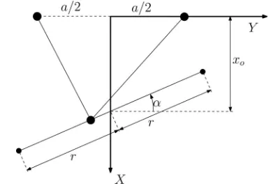
The above derivation requires the prescription of the travel time,Ti, for each of the trajectory segments. The travel time should be chosen in order to maximize the chances of the trajectory to be feasible (no negative tensions). In other words, it should be chosen such that the motion is similar to a periodic motion that is known to always be feasible. Although some periodic motions were studied in [13], they correspond to horizontal, vertical, or circular trajectories. However, the sequence of prescribed points considered here generally involves points that are connected by lines that are neither horizontal nor vertical. In order to obtain insight into such trajectories, a periodic motion along a line segment that makes an angleαwith the horizontal axis is now studied. Consider the periodic symmetric trajectory represented schematically in Fig. 3. The line intersects the x-axis at a distance
Fig. 3. Schematic representation of a periodic symmetric trajectory along a line making an angleαwith they-axis.
x0 from the origin of the coordinate frame, and it is assumed that −π2 < α <π
2. The trajectory can be described mathematically as
x=x0−rsinαsin(ωt), y=rcosαsin(ωt) (30)
tis the time, andris the half-length of the straight line trajectory. Substituting (30) to (32) into inequalities (5) and (6), one obtains, respectively
2. Similarly to what was presented in Section III, two special frequencies can be identified based on (33) and (34), namely
ωs =
gcosα
x0cosα±a2 sinα
. (35)
Depending on the geometric parameters, one of the inequalities is more critical than the other, and the corresponding frequency should be chosen. Using this frequency, the periodic motion is feasible for arbitrary trajectory amplitudesr. The latter frequencyωs is therefore used to determine the travel time for the trajectory segment going from pointito point(i+ 1). Referring to Fig. 3, angleαis computed using
and the corresponding value ofωs is obtained from (35) in whichx0 is taken as
x0 =
xi+xi+ 1
2 . (37)
Finally, since the motion from pointito point(i+ 1)corresponds to a half period, the travel timeTi is computed as
Ti =
π ωs
. (38)
the preceding section will not produce an exact straight line trajectory since the polynomials used for thexandycomponents of the motion are not the same. Nevertheless, heuristically choosing the above travel time is reasonable because the dynamic conditions of the trajectory are close to that of the oscillating motion from which the latter travel time is obtained and the conditions on the coefficients of the polynomials are such that the trajectories will not deviate much from a straight line connecting two consecutive points. As pointed out in the preceding section, a numerical verification of the cable tensions throughout the trajectory must still be performed.
C. Trigonometric Formulation
In order to alleviate the drawbacks of the polynomial formulation proposed above, namely that a numerical verification of the trajectories must be performeda posteriori, an alternative formulation based on trigonometic functions is now proposed. In this formulation, the mo-tion from pointito point(i+ 1)is determined using the following trigonometric expressions:
where parametersri andωi must be adjusted in order to ensure the continuity of the accelerations. The aforementioned functions are se-lected to match the zero velocity conditions at the prescribed points by construction while keeping the algebraic expressions simple. How-ever, it should be pointed out that this formulation does not allow the state of rest (zero velocity and zero acceleration) at a prescribed point. Therefore, the polynomial formulation must be used for the first and last time interval of a given series of prescribed positions in order to start from the state of rest and return to the state of rest at the end of the sequence.
Taking the first two time derivatives of (39) and (40) leads to
˙
which clearly shows that the velocity constraints are satisfied. In ad-dition, the accelerations at the beginning of a given interval are given by
¨
x(0) =Biωi2−4ω2iri, y¨(0) =Diω2i. (49) In order to ensure the continuity of the accelerations, parametersriand
ωican be determined from the latter equations as
ωi =
where y¨i and x¨i are the accelerations in the horizontal and verti-cal directions at target pointiobtained from the previous trajectory segment.
The computation ofωi andri completes the derivation of the tra-jectory for theith trajectory segment. However, it is left to verify that the tensions in the cable remain positive. Because the above trajec-tories are based on trigonometric functions and given the bounds on these functions, it is possible to verify the constraints on the cable ten-sions globally, without having to discretize the trajectory. To this end, the parametric trajectory of (39) and (40) and its time derivatives are substituted into (5) and (6), leading to
V1(t) =E1i+F1icos(ωit) +G1icos(ωit) cos(2ωit)
wheregis the gravitational acceleration, andathe horizontal distance between the attachment points of the cables, as defined in Section II. The expressions on the left-hand side of inequalities (51) and (52) are periodic functions. Hence, in order to ensure that these expressions satisfy the inequalities at all times, it suffices to show that their extrema satisfy the constraints. Differentiating the expressions of (51) and (52) with respect to time and setting the derivative to zero, one obtains
sin(ωit)[(Gj i−Fj i)ωi−4Hj iωicos(ωit)
−6Gj iωicos2(ωit)] = 0, j= 1,2 (60)
with0≤t≤ ωπ
i. Each of the two equations given in (60) leads to four solutions, notedtj k, j= 1,2, k= 1, . . . ,4. Indeed two solutions are
These two solutions correspond to the initial and final points of theith trajectory segment. The other two solutions are obtained by solving the quadratic equation incos(ωit)appearing in (60), which leads to
Fig. 4. Circular trajectory performed by the prototype witha=0.79 m, r= 0.8 m, x0=2 m, andωn =2.21 s−1.
The four solutions corresponding to the extrema ofV1(t)are then sub-stituted into (51), and similarly the four extrema ofV2(t)are substituted into (52), leading to
E1i+F1i+G1i+H1i >0 (65)
E1i−F1i−G1i+H1i >0 (66)
E2i+F2i+G2i+H2i <0 (67)
E2i−F2i−G2i+H2i <0 (68)
V1(t1 3)>0 (69)
V1(t1 4)>0 (70)
V2(t2 3)<0 (71)
V2(t2 4)<0. (72)
The above eight conditions are time independent since they correspond to the extrema. If these eight conditions are satisfied, it can be guaran-teed that the complete trajectory is feasible with positive cable tensions. Therefore, there is no need to discretize the trajectory in order to verify feasibility.
V. EXAMPLETRAJECTORIES ANDEXPERIMENTALVALIDATION A prototype of a two-dof planar cable-suspended robot was devel-oped in order to validate the trajectory planning techniques experi-mentally. The prototype is shown in Fig. 4, where it is performing a circular trajectory that extends beyond the static workspace. The dis-tance between the cable attachment points on the frame isa=0.79 m and the mass of the end effector ism=0.196 kg. Two servo-controlled winches are used to control the length of the cables. In [13], periodic trajectories were developed for a two-dof planar cable-suspended robot including vertical oscillations, horizontal oscillations (described previ-ously in Section III), and circular motions. These periodic trajectories were implemented on the prototype, and they are demonstrated in the first multimedia extension of this paper (seeExtension1-periodic.wmv
as supplementary material).
A. Polynomial Trajectories
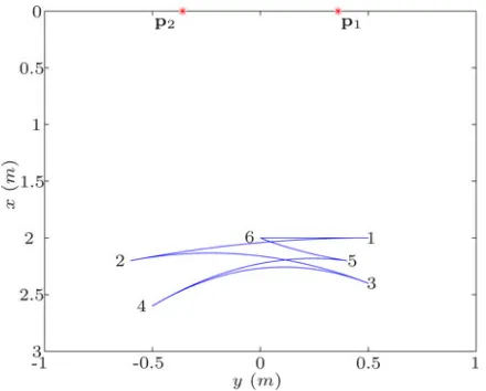
The polynomial point-to-point trajectory-planning technique pre-sented in this paper was tested on the prototype. An example trajectory is described as a set of target points in Fig. 5, where the initial and final points coincide (point 15). The robot is requested to start from a refer-ence configuration located on the central axis of the static workspace (x= 2, y= 0)and to then sequentially proceed to the target points.
Based on the polynomial formulation, the travel times are computed for each trajectory segment using (38), and the fifth-degree polynomi-als of (14) and (21) are used to ensure continuous accelerations. The
Fig. 5. Target points and Cartesian trajectory obtained with the polynomial formulation.
Fig. 6. Tensions in the cables for the trajectory obtained with the polynomial formulation.
Fig. 7. Cartesian velocities for the trajectory obtained with the polynomial formulation.
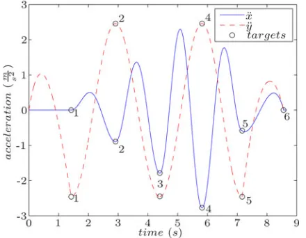
Fig. 8. Cartesian accelerations for the trajectory obtained with the polynomial formulation.
several consecutive intervals. Finally, Fig. 8 shows the components of the acceleration of the end effector. It can be observed that the acceler-ations are continuous, as prescribed. In addition, it can be observed that the acceleration in the horizontal direction reaches a maximum when the target points are reached (zero velocity), while the acceleration in the vertical direction is equal to zero at the target points (zero velocity and acceleration).
Finally, a video demonstrating an example point-to-point tra-jectory is presented in the second multimedia extension (see
Extension2-point-to-point.wmvas supplementary material). The tra-jectory demonstrated in the video was produced using the polynomial formulation described in this paper. It can be observed in the video that the trajectories are smooth, that the target points are properly reached and that tension is maintained in the cables. Prescribing a zero velocity and acceleration in the vertical direction at the target points helps to ensure smoothness. In addition, it can be observed that the travel time between two consecutive points is adjusted according to the position of the latter points. Indeed, referring to (35) and (38), it can be inferred that when the robot is operating closer to the attachment points of the cables (higher in the workspace),x0becomes smaller, which increases the special frequency and, therefore, reduces the travel time. Hence, the robot tends to move more swiftly, as observed in the resulting trajectory and in the video. This behavior is somewhat intuitive and
Fig. 9. Target points and Cartesian trajectory obtained with the trigonometric formulation.
Fig. 10. Tensions in the cables for the trajectory obtained with the trigono-metric formulation.
can be considered an effective exploitation of the dynamics of the robot.
B. Harmonic Trajectories
An example trajectory based on the formulation using trigonometric functions is now presented, which was also tested on the prototype. The trajectory is described as a set of target points in Fig. 9, where the initial and final points coincide (point 6). Similarly to the polynomial trajectory, the robot is requested to start from a reference configuration located on the central axis of the static workspace(x= 2, y= 0)and to then sequentially proceed to the target points.
Fig. 11. Cartesian velocities for the trajectory obtained with the trigonometric formulation.
Fig. 12. Cartesian accelerations for the trajectory obtained with the trigono-metric formulation.
The tensions are continuous and always positive. As opposed to the polynomial trajectory, no discretization was required in order to guar-antee that the trajectory based on trigonometric functions is feasible (positive tensions). Indeed, only the extrema of the trajectory segments need to be tested. Fig. 11 shows the velocity components of the end effector for the trajectory. The velocity components are both zero at the target points, as prescribed by construction of the trigonometric trajec-tories. However, as opposed to the case of the polynomial trajectories, the acceleration in the vertical direction (x-direction) is not prescribed to be zero at the target points, which makes the velocity profile look more like a harmonic function. Finally, Fig. 12 shows the components of the acceleration of the end effector. It can be observed that the accel-erations are continuous, as prescribed. In addition, as opposed to the polynomial trajectory, the acceleration in the vertical direction (x¨) is in general not zero at the target points.
VI. CONCLUSION
This paper addressed the dynamic trajectory planning of two-dof cable-suspended parallel mechanisms for point-to-point motion. The trajectories to be performed are prescribed as a set of target points to be reached with zero velocity. This type of trajectory is of practical interest for applications in which the working range of the mechanism
extends beyond its footprint. Two approaches were proposed. In the first approach, polynomial trajectories are designed in order to ensure the continuity of the accelerations throughout the trajectory. The travel time between two consecutive points is adjusted based on the math-ematical analysis of periodic point-to-point motion. This approach, although somewhat heuristic, produces feasible trajectories for a va-riety of possible consecutive target points. In the second approach, trigonometric functions are used to connect the target points while en-suring continuity of the accelerations. The advantage of the second approach is that the feasibility (positive cable tensions) can be verified using simple algebraic expressions and does not require a discretization of the trajectory. On the other hand, the second approach may fail to connect prescribed points that can be successfully produced with the first approach. Therefore, each of the approaches has its advantages and drawbacks. An experimental validation of the polynomial trajectories is demonstrated in the accompanying videos. Although not shown here, the results obtained with the trigonometric approach are visually very similar. The experiments show that the proposed approaches are feasi-ble, stafeasi-ble, and robust. Indeed, it can be observed that the mechanism is capable of performing point-to-point trajectories very effectively.
This study opens the avenue to using cable-suspended robots beyond their static workspace. Current study includes the extension of the proposed approaches to 3-dof cable-suspended robots, such as those studied in [14], and the development of a constructive method that would allow one to determine the set of target points that can be attained with positive cable tensions from a given point in the Cartesian workspace.
VII. MULTIMEDIAEXTENSIONS
1) Extension1-periodic.wmv—Experimental demonstration on
the prototype of periodic trajectories: vertical oscillations, hori-zontal oscillations, and circular motions.
2) Extension2-point-to-point.wmv—Experimental
demonstra-tion on the prototype of point-to-point polynomial trajectories.
REFERENCES
[1] S. Kawamura, W. Choe, S. Tanaka, and S. Pandian, “Development of an ultrahigh speed robot FALCON using wire drive system,” inProc. IEEE Int. Conf. Robot. Autom., Nagoya, Japan, May 21–27, 1995, pp. 215–220. [2] S. Tadokoro, Y. Murao, M. Hiller, R. Murata, H. Kohkawa, and T. Matsushima, “A motion base with 6-dof by parallel cable drive ar-chitecture,”IEEE/ASME Trans. Mechatron., vol. 7, no. 2, pp. 115–123, Jun. 2002.
[3] J. Albus, R. Bostelman, and N. Dagalakis, “The NIST robocrane,”J. Robot. Syst., vol. 10, no. 5, pp. 709–724, 1993.
[4] J. Pusey, A. Fattah, S. Agrawal, and E. Messina, “Design and workspace analysis of a 6-6 cable-suspended parallel robot,”Mech. Mach. Theory, vol. 39, pp. 761–778, 2004.
[5] C. Gosselin and S. Bouchard, “A gravity-powered mechanism for extend-ing the workspace of a cable-driven parallel mechanism: Application to the appearance modelling of objects,”Int. J. Autom. Technol., vol. 4, no. 4, pp. 372–379, Jul. 2010.
[6] L. L. Cone, “Skycam, an aerial robotic camera system,”Byte, pp. 122–132, Oct. 1985.
[7] A. T. Riechel and I. Ebert-Uphoff, “Force-feasible workspace analysis for underconstrained, point-mass cable robots,” inProc. IEEE Int. Conf. Robot. Autom., New Orleans, LA, USA, Apr. 26–May 1 2004, pp. 4956– 4962.
[10] D. Zanotto, G. Rosati, and S. K. Agrawal, “Modeling and control of a 3-DOF pendulum-like manipulator,” inProc. IEEE Int. Conf. Robot. Au-tom., Shanghai, China, May 9–13, 2011, pp. 3964–3969.
[11] N. Zoso and C. Gosselin, “Point-to-point motion planning of a parallel 3-DOF underactuated cable-suspended robot,” inProc. IEEE Int. Conf. Robot. Autom., St. Paul, MN, USA, May 14–18, 2012, pp. 2325–2330. [12] G. Barrette and C. Gosselin, “Determination of the dynamic workspace
of cable-driven planar parallel mechanisms,”ASME J. Mech. Design, vol. 127, no. 2, pp. 242–248, 2005.
[13] C. Gosselin, P. Ren, and S. Foucault, “Dynamic trajectory planning of a two-DOF cable-suspended parallel robot,” inProc. IEEE Int. Conf. Robot. Autom., St. Paul, MN, USA, pp. 1476–1481, May 14–18, 2012. [14] C. Gosselin, “Global planning of dynamically feasible trajectories for
three-dof spatial cable-suspended parallel robots,” inProc. 1st Int. Conf. Cable-Driven Parallel Robots, Stuttgart, Germany, Sep. 2–4, 2012, pp. 3– 22.
[15] C. Gosselin and A. Hadj-Messaoud, “Automatic planning of smooth tra-jectories for pick-and-place operations,”ASME J. Mech. Design, vol. 115, no. 3, pp. 450–456, 1993.
A New Nonlinear Model of Contact Normal Force
Morteza Azad and Roy Featherstone
Abstract—This paper presents a new nonlinear model of the normal force that arises during compliant contact between two spheres, or between a sphere and a flat plate. It differs from a well-known existing model by only a single term. The advantage of the new model is that it accurately predicts the measured values of the coefficient of restitution between spheres and plates of various materials, whereas other models do not.
Index Terms—Animation and simulation, compliant contact model, non-linear damping, normal force.
I. INTRODUCTION
Since robots usually make contact with their environment during the execution of their tasks (e.g., grasping, walking, rolling, etc.), modeling the contact is an unavoidable part of most studies in this field. Two major forces appear during contact: the normal force and the friction force. In this paper, we focus on the normal force and introduce a new model for calculating it. This new model agrees well with existing measurements of the coefficient of restitution between spheres and plates of various materials.
Contact models can be classified into two types: rigid and com-pliant [3]. The model presented in this paper is comcom-pliant. The key difference is that compliant models assume a small amount of local deformation at the contact, which allows the contact forces to be ex-pressed as functions of local position and velocity variables. This fea-ture makes it relatively easy to incorporate a compliant contact model into a dynamics simulator.
Most previous studies of compliant contact models have considered the contact between two spheres, or between a sphere and a flat plate [2], [5], [8], [10]. For example, Hunt and Crossley [5] modeled the ground as a nonlinear spring–damper pair at the contact point with the sphere,
Manuscript received August 1, 2013; accepted November 21, 2013. Date of publication December 19, 2013; date of current version June 3, 2014. This paper was recommended for publication by Associate Editor J. Dai and Editor B. J. Nelson upon evaluation of the reviewers’ comments.
M. Azad is with the School of Engineering, The Australian National University, Canberra, Acton, A.C.T. 0200, Australia (e-mail: morteza.azad@ anu.edu.au).
R. Featherstone is a Visiting Professor with the Department Advanced Robotics, Istituto Italiano di Tecnologia, Genova 16163, Italy (e-mail: [email protected]).
Digital Object Identifier 10.1109/TRO.2013.2293833
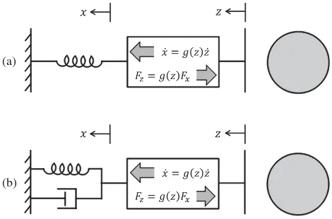
(a)
(b)
Fig. 1. Nonlinear (a) elastic and (b) viscoelastic models of contact in which the nonlinearity is encapsulated in a gearbox with a position-dependent gear ratio ofg(z).
and introduced a nonlinear equation for the normal force between a sphere and the ground as
F=kzn+λzpz˙q (1)
wherezis the deformation variable, which is defined as the penetration distance of the undeformed sphere into the undeformed ground,z˙is the rate of deformation,kandλare the coefficients of the spring and damper, respectively, andn,p,and qare constant parameters. They chose the values of these parameters asn= 3
2 (to get similar results to Hertz’s theory [6]),p= 3
2, andq= 1(to be able to determine the value ofλwith respect tokconveniently), resulting in the equation
F=kz32 +λz32z.˙ (2)
This model has since appeared in [8] and [10], and has become well known in the robotics community. We shall refer to it as the Hunt/Crossley model. Following a different line of reasoning, Lee and Wang [9] obtained a model identical to (2), but withp= 1instead of 3
2. Our new model also differs from (2) only in the value ofp, which we show has to bep= 1
2.
In the remainder of this paper, we first derive the new model and then test it against experimentally measured values of the coefficient of restitution between spheres and plates of various materials. It is shown that the new model accurately fits the experimental data, whereas the Hunt/Crossley model does not. The new model is based on an idea that appeared originally in [1], which studied the contact between a rigid sphere and a compliant plate.
II. CONTACTFORCEMODEL
The contact force in (1) is the sum of an elastic component and a dissipative component. The expressionkz32 in (2) is the elastic force
predicted by Hertz’s theory for contact between a sphere and a plate, and is known to be correct. As Hertz’s theory is based on an assumption of linear elasticity in the contacting solids, it follows that the nonlinearity in the elastic force expression is due to the nonlinear geometry at the contact (i.e., the curved surface of the sphere).
We can model the elastic contact force with a linear spring and a nonlinear gearbox, as shown in Fig. 1(a). The spring represents the lumped elasticity of the contacting bodies, and its stiffnessKdepends on the material properties of the contacting bodies. The gearbox has a deformation-dependent gear ratio ofg(z)and represents the nonlinear variation of contact area and strain distribution withz.