John D. Anderson, Jr., University of Maryland,Consulting Editor
Hypersonic and High Temperature Gas Dynamics
Advanced Strength and Applied Stress Analysis
C¸ engel and Cimbala
Fluid Mechanics
Space Propulation Analysis and Design
Hyer
Stress Analysis of Fiber-Reinforced Composite Materials
Flight Stability and Automatic Control
Oosthuizen
Stresses in Plates and Shells
T
of the twentieth century. Along with this came the rise of aeronautical engineering as an exciting, new, distinct discipline. College courses in aeronautical engineering were offered as early as 1914 at the University of Michigan and at MIT. Michigan was the first university to establish an aero-nautics department with a four-year degree-granting program in 1916; by 1926 it had graduated over one hundred students. The need for substantive textbooks in various areas of aeronautical engineering became critical. Rising to this demand, McGraw-Hill became one of the first publishers of aeronautical engineering text-books, starting withAirplane Design and Constructionby Ottorino Pomilio in 1919, and the classic and definitive textAirplane Design: Aerodynamicsby the iconic Edward P. Warner in 1927. Warner’s book was a watershed in aeronautical engineering textbooks.Since then, McGraw-Hill has become the time-honored publisher of books in aeronautical engineering. With the advent of high-speed flight after World War II and the space program in 1957, aeronautical and aerospace engineering grew to new heights. There was, however, a hiatus that occurred in the 1970s when aerospace engineering went through a transition, and virtually no new books in the field were published for almost a decade by anybody. McGraw-Hill broke this hiatus with the foresight of its Chief Engineering Editor, B.J. Clark, who was instrumental in the publication ofIntroduction to Flightby John Anderson. First published in 1978,Introduction to Flightis now in its 6th edition. Clark’s bold decision was followed by McGraw-Hill riding the crest of a new wave of students and activity in aerospace engineering, and it opened the flood-gates for new textbooks in the field.
In 1988, McGraw-Hill initiated its formal series in Aeronautical and Aerospace Engineering, gathering together under one roof all its existing texts in the field, and soliciting new manuscripts. This author is proud to have been made the consulting editor for this series, and to have contributed some of the titles. Starting with eight books in 1988, the series now embraces 24 books cov-ering a broad range of discipline in the field. With this, McGraw-Hill continues its tradition, started in 1919, as the premier publisher of important textbooks in aeronautical and aerospace engineering.
John D. Anderson, Jr.
Curator of Aerodynamics National Air and Space Museum Smithsonian Institution
and
Published by McGraw-Hill, a business unit of The McGraw-Hill Companies, Inc., 1221 Avenue of the Americas, New York, NY 10020. Copyright © 2011 by The McGraw-Hill Companies, Inc. All rights reserved. Previous editions © 2007, 2001, 1991 and 1984. No part of this publication may be reproduced or distributed in any form or by any means, or stored in a database or retrieval system, without the prior written consent of The McGraw-Hill Companies, Inc., including, but not limited to, in any network or other electronic storage or transmission, or broadcast for distance learning.
Some ancillaries, including electronic and print components, may not be available to customers outside the United States.
This book is printed on acid-free paper.
1 2 3 4 5 6 7 8 9 0 DOC/DOC 1 0 9 8 7 6 5 4 3 2 1 0 ISBN 978-0-07-339810-5
MHID 0-07-339810-1
Global Publisher: Raghothaman Srinivasan Senior Sponsoring Editor: Bill Stenquist Director of Development: Kristine Tibbetts Developmental Editor: Lorraine K. Buczek Senior Marketing Manager: Curt Reynolds Senior Project Manager: Jane Mohr Production Supervisor: Susan K. Culberston Design Coordinator: Brenda A. Rolwes
Cover Designer: Studio Montage, St. Louis, Missouri (USE) Cover Image: © U.S. Navy photo
Lead Photo Research Coordinator: Carrie K. Burger Compositor: Aptara, Inc.
Typeface: 10.5/12 Times Roman Printer: R. R. Donnelley
All credits appearing on page or at the end of the book are considered to be an extension of the copyright page.
The white cloud that you see in the flow over the top of the F-22 on the cover of this book is due to water vapor condensation occurring through the supersonic expansion waves on the top of the airplane. This white cloud is abruptly terminated when the flow subsequently passes through the trailing-edge shock waves behind the airplane. A detailed physical explanation of this flow can be found in Problem 9.21 at the end of Chapter 9.
Library of Congress Cataloging-in-Publication Data
Anderson, John David.
Fundamentals of aerodynamics / John D. Anderson, Jr. — 5th ed.
p. cm. — (McGraw-Hill series in aeronautical and aerospace engineering) Includes bibliographical references and index.
ISBN-13: 978-0-07-339810-5 ISBN-10: 0-07-339810-1 1. Aerodynamics. I. Title. TL570.A677 2010
629.132′3—dc22 2009048907
a bachelor of aeronautical engineering degree. From 1959 to 1962, he was a lieutenant and task scientist at the Aerospace Research Laboratory at Wright-Patterson Air Force Base. From 1962 to 1966, he attended the Ohio State Univer-sity under the National Science Foundation and NASA Fellowships, graduating with a Ph.D. in aeronautical and astronautical engineering. In 1966, he joined the U.S. Naval Ordnance Laboratory as Chief of the Hypersonics Group. In 1973, he became Chairman of the Department of Aerospace Engineering at the Uni-versity of Maryland, and since 1980 has been professor of Aerospace Engineer-ing at the University of Maryland. In 1982, he was designated a DistEngineer-inguished Scholar/Teacher by the University. During 1986–1987, while on sabbatical from the University, Dr. Anderson occupied the Charles Lindbergh Chair at the Na-tional Air and Space Museum of the Smithsonian Institution. He continued with the Air and Space Museum one day each week as their Special Assistant for Aero-dynamics, doing research and writing on the history of aerodynamics. In addition to his position as professor of aerospace engineering, in 1993, he was made a full faculty member of the Committee for the History and Philosophy of Science and in 1996 an affiliate member of the History Department at the University of Maryland. In 1996, he became the Glenn L. Martin Distinguished Professor for Education in Aerospace Engineering. In 1999, he retired from the University of Maryland and was appointed Professor Emeritus. He is currently the Curator for Aerodynamics at the National Air and Space Museum, Smithsonian Institution.
Dr. Anderson has published 10 books:Gasdynamic Lasers: An Introduction,
Academic Press (1976), and under McGraw-Hill,Introduction to Flight(1978, 1984, 1989, 2000, 2005, 2008),Modern Compressible Flow(1982, 1990, 2003),
Fundamentals of Aerodynamics(1984, 1991, 2001, 2007),Hypersonic and High Temperature Gas Dynamics(1989),Computational Fluid Dynamics: The Basics with Applications(1995),Aircraft Performance and Design(1999),A History of Aerodynamics and Its Impact on Flying Machines,Cambridge University Press (1997 hardback, 1998 paperback),The Airplane: A History of Its Technology,
American Institute of Aeronautics and Astronautics (2003), andInventing Flight,
Johns Hopkins University Press (2004). He is the author of over 120 papers on radiative gasdynamics, reentry aerothermodynamics, gasdynamic and chemical lasers, computational fluid dynamics, applied aerodynamics, hypersonic flow, and the history of aeronautics. Dr. Anderson is inWho’s Who in America. He is an Honorary Fellow of the American Institute of Aeronautics and Astronautics (AIAA). He is also a fellow of the Royal Aeronautical Society, London. He is a member of Tau Beta Pi, Sigma Tau, Phi Kappa Phi, Phi Eta Sigma, The American
P A R T
1
Fundamental Principles
1
Chapter
1
Aerodynamics: Some Introductory
Thoughts 3
1.1 Importance of Aerodynamics: Historical
Examples 5
1.2 Aerodynamics: Classification and Practical Objectives 11
1.3 Road Map for This Chapter 15 1.4 Some Fundamental Aerodynamic
Variables 15
1.4.1 Units 18
1.5 Aerodynamic Forces and Moments 19 1.6 Center of Pressure 32
1.7 Dimensional Analysis: The Buckingham Pi Theorem 34
1.8 Flow Similarity 41
1.9 Fluid Statics: Buoyancy Force 52 1.10 Types of Flow 62
1.10.1 Continuum Versus Free Molecule Flow 62
1.10.2 Inviscid Versus Viscous Flow 62 1.10.3 Incompressible Versus Compressible
Flows 64
1.10.4 Mach Number Regimes 64
1.11 Viscous Flow: Introduction to Boundary Layers 68
Variations 75
1.13 Historical Note: The Illusive Center of Pressure 89
2.1 Introduction and Road Map 104 2.2 Review of Vector Relations 105
2.2.1 Some Vector Algebra 106 2.2.2 Typical Orthogonal Coordinate
Systems 107
2.2.3 Scalar and Vector Fields 110 2.2.4 Scalar and Vector Products 110 2.2.5 Gradient of a Scalar Field 111 2.2.6 Divergence of a Vector Field 113 2.2.7 Curl of a Vector Field 114 2.2.8 Line Integrals 114 2.2.9 Surface Integrals 115 2.2.10 Volume Integrals 116
2.2.11 Relations Between Line, Surface, and Volume Integrals 117 2.2.12 Summary 117
2.3 Models of the Fluid: Control Volumes and Fluid Elements 117
2.3.1 Finite Control Volume Approach 118
2.3.2 Infinitesimal Fluid Element Approach 119
2.3.3 Molecular Approach 119
2.3.4 Physical Meaning of the Divergence of Velocity 120
2.3.5 Specification of the Flow Field 121
2.4 Continuity Equation 125
2.5 Momentum Equation 130
2.6 An Application of the Momentum Equation: Drag of a Two-Dimensional Body 135
2.6.1 Comment 144
2.7 Energy Equation 144 2.8 Interim Summary 149 2.9 Substantial Derivative 150 2.10 Fundamental Equations in Terms
of the Substantial Derivative 156 2.11 Pathlines, Streamlines, and Streaklines
of a Flow 158
2.12 Angular Velocity, Vorticity, and Strain 163 2.13 Circulation 174
2.14 Stream Function 177 2.15 Velocity Potential 181
2.16 Relationship Between the Stream Function and Velocity Potential 184
2.17 How Do We Solve the Equations? 185
2.17.1 Theoretical (Analytical) Solutions 185 2.17.2 Numerical Solutions—Computational
Fluid Dynamics (CFD) 187 2.17.3 The Bigger Picture 194
2.18 Summary 194
3.1 Introduction and Road Map 204
3.2 Bernoulli’s Equation 207
3.3 Incompressible Flow in a Duct: The Venturi and Low-Speed Wind Tunnel 211
3.4 Pitot Tube: Measurement of Airspeed 224
3.5 Pressure Coefficient 233
3.6 Condition on Velocity for Incompressible
Flow 235
3.7 Governing Equation for Irrotational, Incompressible Flow: Laplace’s Equation 236
3.7.1 Infinity Boundary Conditions 239 3.7.2 Wall Boundary Conditions 239
3.8 Interim Summary 240
3.9 Uniform Flow: Our First Elementary
Flow 241
3.10 Source Flow: Our Second Elementary
Flow 243
3.11 Combination of a Uniform Flow with a Source and Sink 247
3.12 Doublet Flow: Our Third Elementary
Flow 251
3.13 Nonlifting Flow over a Circular Cylinder 253
3.14 Vortex Flow: Our Fourth Elementary
Flow 262
3.15 Lifting Flow over a Cylinder 266 3.16 The Kutta-Joukowski Theorem and the
Generation of Lift 280
3.17 Nonlifting Flows over Arbitrary Bodies: The Numerical Source Panel
Method 282
3.18 Applied Aerodynamics: The Flow over a Circular Cylinder—The Real Case 292 3.19 Historical Note: Bernoulli and Euler—The
Origins of Theoretical Fluid
Dynamics 300
3.20 Historical Note: d’Alembert and His
Paradox 305
3.21 Summary 306
4.4 Philosophy of Theoretical Solutions for Low-Speed Flow over Airfoils: The Vortex Sheet 325
4.5 The Kutta Condition 330
4.5.1 Without Friction Could We Have Lift? 334
4.6 Kelvin’s Circulation Theorem and the Starting Vortex 334
4.7 Classical Thin Airfoil Theory: The Symmetric Airfoil 338
4.8 The Cambered Airfoil 348
4.9 The Aerodynamic Center: Additional Considerations 357
4.10 Lifting Flows over Arbitrary Bodies: The Vortex Panel Numerical Method 361
4.11 Modern Low-Speed Airfoils 367 4.12 Viscous Flow: Airfoil Drag 371
4.12.1 Estimating Skin-Friction Drag:
4.13 Applied Aerodynamics: The Flow over an Airfoil—The Real Case 387 4.14 Historical Note: Early Airplane
Design and the Role of Airfoil Thickness 398
4.15 Historical Note: Kutta, Joukowski, and the Circulation Theory
5.3.1 Elliptical Lift Distribution 430 5.3.2 General Lift Distribution 435 5.3.3 Effect of Aspect Ratio 438 5.3.4 Physical Significance 444
5.4 A Numerical Nonlinear Lifting-Line
Method 453
5.5 The Lifting-Surface Theory and the Vortex Lattice Numerical Method 457
5.6 Applied Aerodynamics: The Delta
Wing 464
5.7 Historical Note: Lanchester and Prandtl—The Early Development of 6.4 Flow over A Sphere 492
6.4.1 Comment on the Three-Dimensional Relieving Effect 494
6.5 General Three-Dimensional Flows: Panel Techniques 495
6.7 Applied Aerodynamics: Airplane Lift and Drag 500
6.7.1 Airplane Lift 500 6.7.2 Airplane Drag 502
6.7.3 Application of Computational Fluid Dynamics for the Calculation of Lift and Drag 507
7.2 A Brief Review of Thermodynamics 518
7.2.1 Perfect Gas 518
7.2.2 Internal Energy and Enthalpy 518 7.2.3 First Law of Thermodynamics 523 7.2.4 Entropy and the Second Law of
Thermodynamics 524 7.2.5 Isentropic Relations 526
7.3 Definition of Compressibility 530 7.4 Governing Equations for Inviscid,
Compressible Flow 531 7.5 Definition of Total (Stagnation)
Conditions 533
7.6 Some Aspects of Supersonic Flow: Shock
Waves 540
7.7 Summary 544
7.8 Problems 546
Chapter
8
Normal Shock Waves and Related Topics 549 8.1 Introduction 550
8.2 The Basic Normal Shock Equations 551
8.3 Speed of Sound 555
8.3.1 Comments 563
8.4 Special Forms of the Energy Equation 564
8.5 When Is A Flow Compressible? 572 8.6 Calculation of Normal Shock-Wave
Properties 575
8.6.1 Comment on the Use of Tables to Solve Compressible Flow Problems 590
8.7 Measurement of Velocity in a Compressible
Flow 591
8.7.1 Subsonic Compressible Flow 591 8.7.2 Supersonic Flow 592
8.8 Summary 596
8.9 Problems 599
Chapter
9
Oblique Shock and Expansion Waves 601
9.1 Introduction 602
9.2 Oblique Shock Relations 608 9.3 Supersonic Flow over Wedges
and Cones 622
9.3.1 A Comment on Supersonic Lift and Drag Coefficients 625
9.4 Shock Interactions and Reflections 626 9.5 Detached Shock Wave in Front of a Blunt
Body 632
9.5.1 Comment on the Flow Field behind a Curved Shock Wave: Entropy Gradients and Vorticity 636
9.6 Prandtl-Meyer Expansion Waves 636 9.7 Shock-Expansion Theory: Applications to
Supersonic Airfoils 648 9.8 A Comment on Lift and Drag
Coefficients 652
9.9 The X-15 and Its Wedge Tail 652 9.10 Viscous Flow: Shock-Wave/
Boundary-Layer Interaction 657 9.11 Historical Note: Ernst Mach—A
and Wind Tunnels 669 10.1 Introduction 670 10.2 Governing Equations for
Quasi-One-Dimensional Flow 672 10.3 Nozzle Flows 681
10.3.1 More on Mass Flow 695
10.4 Diffusers 696
10.5 Supersonic Wind Tunnels 698 10.6 Viscous Flow: Shock-Wave/
Subsonic Compressible Flow over Airfoils:
Linear Theory 711
11.1 Introduction 712
11.2 The Velocity Potential Equation 714 11.3 The Linearized Velocity Potential
Equation 717
11.4 Prandtl-Glauert Compressibility Correction 722
11.5 Improved Compressibility Corrections 727
11.6 Critical Mach Number 728
11.6.1 A Comment on the Location of Minimum Pressure (Maximum Velocity) 737
11.7 Drag-Divergence Mach Number: The Sound Barrier 737
11.8 The Area Rule 745
11.9 The Supercritical Airfoil 747 11.10 CFD Applications: Transonic Airfoils
and Wings 749
Swept-Wing Concept 764 11.14 Historical Note: Richard T.
Whitcomb—Architect of the Area Rule and the Supercritical Wing 773
11.15 Summary 774
11.16 Problems 776
Chapter
12
Linearized Supersonic Flow 779 12.1 Introduction 780
12.2 Derivation of the Linearized Supersonic Pressure Coefficient Formula 780 12.3 Application to Supersonic Airfoils 784 12.4 Viscous Flow: Supersonic Airfoil
Drag 790
12.5 Summary 793
12.6 Problems 794
Chapter
13
Introduction to Numerical Techniques for Nonlinear Supersonic Flow 797
13.1 Introduction: Philosophy of Computational Fluid Dynamics 798
13.2 Elements of the Method of Characteristics 800
13.2.1 Internal Points 806 13.2.2 Wall Points 807
13.3 Supersonic Nozzle Design 808 13.4 Elements of Finite-Difference
Methods 811
13.5 The Time-Dependent Technique: Application to Supersonic Blunt Bodies 818
13.5.1 Predictor Step 822 13.5.2 Corrector Step 822
13.6 Flow over Cones 826
13.6.1 Physical Aspects of Conical Flow 827
13.6.2 Quantitative Formulation 828 13.6.3 Numerical Procedure 833
13.6.4 Physical Aspects of Supersonic Flow Over Cones 834
13.7 Summary 837
13.8 Problem 838
Chapter
14
Elements of Hypersonic Flow 839 14.1 Introduction 840
14.2 Qualitative Aspects of Hypersonic
Flow 841
14.3 Newtonian Theory 845
14.4 The Lift and Drag of Wings at Hypersonic Speeds: Newtonian Results for a Flat Plate at Angle of Attack 849
14.4.1 Accuracy Considerations 856
14.5 Hypersonic Shock-Wave Relations and Another Look at Newtonian Theory 860
14.6 Mach Number Independence 864 14.7 Hypersonics and Computational Fluid
Dynamics 866
14.8 Hypersonic Viscous Flow: Aerodynamic Heating 869
14.8.1 Aerodynamic Heating and Hypersonic Flow—the Connection 869
14.8.2 Blunt versus Slender Bodies in Hypersonic Flow 871 14.8.3 Aerodynamic Heating to a
Blunt Body 874
Introduction to the Fundamental Principles and Equations of Viscous Flow 893 15.1 Introduction 894
15.2 Qualitative Aspects of Viscous
Flow 895
15.3 Viscosity and Thermal Conduction 903 15.4 The Navier-Stokes Equations 908 15.5 The Viscous Flow Energy Equation 912 15.6 Similarity Parameters 916
15.7 Solutions of Viscous Flows: A Preliminary Discussion 920
15.8 Summary 923
15.9 Problems 925
Chapter
16
A Special Case: Couette Flow 927 16.1 Introduction 927
16.2 Couette Flow: General Discussion 928 16.3 Incompressible (Constant Property)
Couette Flow 932
16.3.1 Negligible Viscous Dissipation 938 16.3.2 Equal Wall Temperatures 939 16.3.3 Adiabatic Wall Conditions (Adiabatic
Method 952
16.4.3 Results for Compressible Couette Flow 956
16.4.4 Some Analytical Considerations 958
16.5 Summary 963
Chapter
17
Introduction to Boundary Layers 965 17.1 Introduction 966
17.2 Boundary-Layer Properties 968 17.3 The Boundary-Layer Equations 974 17.4 How Do We Solve the Boundary-Layer
Equations? 977
17.5 Summary 979
Chapter
18
Laminar Boundary Layers 981
18.1 Introduction 981
18.2 Incompressible Flow over a Flat Plate: The Blasius Solution 982
18.3 Compressible Flow over a Flat Plate 989
18.3.1 A Comment on Drag Variation with Velocity 1000
18.4 The Reference Temperature Method 1001
18.4.1 Recent Advances: The Meador-Smart Reference Temperature Method 1004
18.5 Stagnation Point Aerodynamic Heating 1005
18.6 Boundary Layers over Arbitrary Bodies: Finite-Difference Solution 1011
19.2.3 Prediction of Airfoil Drag 1025
19.3 Turbulence Modeling 1025
19.3.1 The Baldwin-Lomax Model 1026
19.4 Final Comments 1028
20.3 Examples of Some Solutions 1033
20.3.1 Flow over a Rearward-Facing Step 1033 20.3.2 Flow over an Airfoil 1033
20.3.3 Flow over a Complete Airplane 1036 20.3.4 Shock-Wave/Boundary-Layer Interaction
1037
20.3.5 Flow over an Airfoil with a Protuberance 1038
20.4 The Issue of Accuracy for the Prediction of Skin Friction Drag 1040
20.5 Summary 1045
Appendix A
Isentropic Flow Properties 1047 Appendix B
Appendix C
Prandtl-Meyer Function and Mach
Angle 1057
Appendix D
Standard Atmosphere, SI Units 1061
Appendix E
Standard Atmosphere, English Engineering
Units 1071
Bibliography 1079
T
and gain his or her immediate interest in the challenging and yet beautiful discipline of aerodynamics. The explanation of each topic is carefully constructed to make sense to the reader. Moreover, the structure of each chapter is tightly or-ganized in order to keep the reader aware of where we are, where we were, and where we are going. Too frequently the student of aerodynamics loses sight of what is trying to be accomplished; to avoid this, I attempt to keep the reader informed of my intent at all times. For example, preview boxes are introduced at the beginning of each chapter. These short sections, literally set in boxes, are to inform the reader in plain language what to expect from each chapter, and why the material is important and exciting. They are primarily motivational; they help to encourage the reader to actually enjoy reading the chapter, therefore enhancing the educational process. In addition, each chapter contains a road map—a block diagram designed to keep the reader well aware of the proper flow of ideas and concepts. The use of preview boxes and chapter road maps are unique features of this book. Also, to help organize the reader’s thoughts, there are special summary sections at the end of most chapters.The material in this book is at the level of college juniors and seniors in aerospace or mechanical engineering. It assumes no prior knowledge of fluid dynamics in general, or aerodynamics in particular. It does assume a familiarity with differential and integral calculus, as well as the usual physics background common to most students of science and engineering. Also, the language of vector analysis is used liberally; a compact review of the necessary elements of vector algebra and vector calculus is given in Chapter 2 in such a fashion that it can either educate or refresh the reader, whatever may be the case for each individual.
This book is designed for a 1-year course in aerodynamics. Chapters 1 to 6 constitute a solid semester emphasizing inviscid, incompressible flow. Chapters 7 to 14 occupy a second semester dealing with inviscid, compressible flow. Finally, Chapters 15 to 20 introduce some basic elements of viscous flow, mainly to serve as a contrast to and comparison with the inviscid flows treated throughout the bulk of the text. Specific sections on viscous flow, however, have been added much earlier in the book in order to give the reader some idea of how the inviscid results are tempered by the influence of friction. This is done by adding self-contained viscous flow sections at the end of various chapters, written and placed in such a way that they do not interfere with the flow of the inviscid flow discussion, but are there to complement the discussion. For example, at the end of Chapter 4 on incompressible inviscid flow over airfoils, there is a viscous flow section that deals
with the prediction of skin friction drag on such airfoils. A similar viscous flow section at the end of Chapter 12 deals with friction drag on high-speed airfoils. At the end of the chapters on shock waves and nozzle flows, there are viscous flow sections on shock-wave/boundary-layer interactions. And so forth.
Other features of this book are:
1. An introduction to computational fluid dynamics as an integral part of the study of aerodynamics. Computational fluid dynamics (CFD) has recently become a third dimension in aerodynamics, complementing the previously existing dimensional of pure experiment and pure theory. It is absolutely necessary that the modern student of aerodynamics be introduced to some of the basic ideas of CFD—he or she will most certainly come face to face with either its “machinery” or its results after entering the professional ranks of practicing aerodynamicists. Hence, such subjects as the source and vortex panel techniques, the method of characteristics, and explicit
finite-difference solutions are introduced and discussed as they naturally arise during the course of our discussion. In particular, Chapter 13 is devoted exclusively to numerical techniques, couched at a level suitable to an introductory aerodynamics text.
2. A chapter is devoted entirely to hypersonic flow. Although hypersonics is at one extreme end of the flight spectrum, it has current important applications to the design of the space shuttle, hypervelocity missiles, planetary entry vehicles, and modern hypersonic atmospheric cruise vehicles. Therefore, hypersonic flow deserves some attention in any modern presentation of aerodynamics. This is the purpose of Chapter 14.
3. Historical notes are placed at the end of many of the chapters. This follows in the tradition of some of my previous textbooks,Introduction to Flight: Its Engineering and History,sixth edition (McGraw-Hill, 2008). andModern Compressible Flow: With Historical Perspective,third edition
(McGraw-Hill, 2003). Although aerodynamics is a rapidly evolving subject, its foundations are deeply rooted in the history of science and technology. It is important for the modern student of aerodynamics to have an
appreciation for the historical origin of the tools of the trade. Therefore, this book addresses such questions as who were Bernoulli, Euler, d’Alembert, Kutta, Joukowski, and Prandtl; how the circulation theory of lift developed; and what excitement surrounded the early development of high-speed aerodynamics. I wish to thank various members of the staff of the National Air and Space Museum of the Smithsonian Institution for opening their extensive files for some of the historical research behind these history sections. Also, a constant biographical reference was theDictionary of Scientific Biography,edited by C. C. Gillespie, Charles Schribner’s Sons, New York, 1980. This 16-volume set of books is a valuable source of biographic information on leading scientists in history.
Because of the extremely favorable comments from readers and users of the first four editions, virtually all the content of the earlier editions has been carried over intact to the present fifth edition. In this edition much new material has been added in order to enhance, update, and expand that covered in the earlier editions. There are 41 new figures, 23 inserts of new material and new sections, many new worked examples, and additional homework problems. In particular, the fifth edition has the followingnew features:
1. A new section in Chapter 6 on airplane lift and drag. The flow over a complete airplane is an important three-dimensional flow. This section, in a chapter on three-dimensional flows, focuses on how to estimate the lift and drag of a complete airplane.
2. A new section in Chapter 9 on the flow field behind a curved shock wave explaining why this flow is rotational.
3. A new section in Chapter 9 that asks the question why does the X-15 hypersonic research vehicle have a wedge tail instead of a slender airfoil section? The answer involves an innovative application of shock-expansion theory, and serves as an interesting design example of the importance of shock waves and expansion waves.
4. A new section highlighting the blended-wing-body configuration. This is a very promising innovative design concept for high-speed subsonic
transports and cargo carriers. This section emphasizes how the principles of subsonic compressible flow discussed in Chapter 11 are applied to the blended wing body.
5. A new historical note on the origin of the swept-wing concept. Who conceived the use of swept wings for high-speed airplanes? Why? This section covers the history of the swept-wing concept and incorporates some newly discovered German design data from World War II.
6. A new section on supersonic flow over cones. This is an important addition to Chapter 13 on numerical techniques for nonlinear supersonic flow, because supersonic flow over cones is a classic example of supersonic aerodynamics. Moreover, this section is an important precursor to a following section on hypersonic waveriders in Chapter 14.
8. A new section on applied hypersonic aerodynamics: hypersonic waveriders, in Chapter 14. Hypersonic waveriders are a viable new configuration for hypersonic vehicles, and this is an extensive discussion of such vehicles – how they are designed and an examination of their aerodynamic advantage. 9. A small part of the existing Part 4 on viscous flow has been shortened and
streamlined. Part 4 was never designed to represent a total course on viscous flow, but rather is included for balance and completeness of the fundamentals of aerodynamics.
10. Many additional new worked examples. When learning new technical material, especially material of a fundamental nature as emphasized in this book, one can never have too many examples of how the fundamentals can be applied to the solution of problems.
11. New homework problems at the end of each chapter, added to those carried over from the fourth edition
All the new additional material not withstanding, the main thrust of this book remains the presentation of the fundamentals of aerodynamics; the new material is simply intended to enhance and support this thrust. I repeat that the book is organized along classical lines, dealing with inviscid incompressible flow, inviscid compressible flow, and viscous flow in sequence. My experience in teaching this material to undergraduates finds that it nicely divides into a two-semester course with Parts 1 and 2 in the first semester, and Parts 3 and 4 in the second semester. Also, I have taught the entire book in a fast-paced, first-semester graduate course intended to introduce the fundamentals of aerodynamics to new graduate students who have not had this material as part of their undergraduate education. The book works well in such a mode.
I would like to thank the McGraw-Hill editorial and production staff for their excellent help in producing this book, especially Lorraine Buczek and Jane Mohr in Dubuque. Also, special thanks go to my long-time friend and associate, Sue Cunningham, whose expertise as a scientific typist is beyond comparison, and who has typed all my book manuscripts for me, including this one, with great care and precision.
I would like to thank the following revision survey participants for their valuable feedback: Lian Duan, Princeton University; Vladimir Golubev, Embry Riddle Aeronautical University; Tej Gupta, Embry Riddle Aeronautical Univer-sity; Serhat Hosder, Missouri University of Science and Technology; Narayanan Komerath, Georgia Institute of Technology; Luigi Martinelli, Princeton Univer-sity; Jim McDaniel, University of Virginia; Jacques C. Richard, Texas A&M Uni-versity; Steven Schneider, Purdue UniUni-versity; Wei Shyy, University of Michigan; and Brian Thurow, Auburn University.
As a final comment, aerodynamics is a subject of intellectual beauty, com-posed and drawn by many great minds over the centuries.Fundamentals of Aero-dynamicsis intended to portray and convey this beauty. Do you feel challenged and interested by these thoughts? If so, then read on, and enjoy!
1
Fundamental Principles
I
n Part 1, we cover some of the basic principles that apply to aerodynamics in general. These are the pillars on which all of aerodynamics is based.Aerodynamics: Some
Introductory Thoughts
The term “aerodynamics” is generally used for problems arising from flight and other topics involving the flow of air.
Ludwig Prandtl, 1949
Aerodynamics: The dynamics of gases, especially atmospheric interactions with moving objects.
The American Heritage Dictionary of the English Language, 1969
PREVIEW BOX
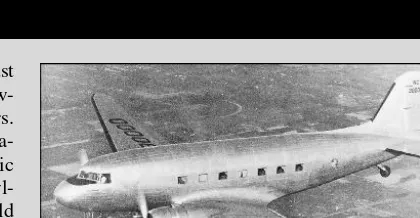
Why learn about aerodynamics? For an answer, just take a look at the following five photographs show-ing a progression of airplanes over the past 70 years. The Douglas DC-3 (Figure 1.1), one of the most fa-mous aircraft of all time, is a low-speed subsonic transport designed during the 1930s. Without a knowl-edge of low-speed aerodynamics, this aircraft would have never existed. The Boeing 707 (Figure 1.2) opened high-speed subsonic flight to millions of pas-sengers beginning in the late 1950s. Without a knowl-edge of high-speed subsonic aerodynamics, most of
us would still be relegated to ground transportation. Figure 1.1 Douglas DC-3 (Courtesy of the American Aviation Historical Society).
Figure 1.2 Boeing 707 (Courtesy of the Harold Andrews Collection).
Figure 1.3 Bell X-1 (Courtesy of the National Air and Space Museum).
Figure 1.4 Lockheed F-104 (Courtesy of the Harold Andrews Collection).
The Bell X-1 (Figure 1.3) became the first piloted air-plane to fly faster than sound, a feat accomplished with Captain Chuck Yeager at the controls on Oc-tober 14, 1947. Without a knowledge of transonic aerodynamics (near, at, and just above the speed of sound), neither the X-1, nor any other airplane, would have ever broken the sound barrier. The Lockheed F-104 (Figure 1.4) was the first supersonic airplane
Figure 1.5 Lockheed-Martin F-22 (Courtesy of the Harold Andrews Collection).
Figure 1.6 Blended wing body (NASA).
thrust by gas turbine jet engines and rocket engines, and the movement of air through building heater and air-conditioning systems are just a few other exam-ples of the application of aerodynamics. The material in this book is powerful stuff—important stuff. Have fun reading and learning about aerodynamics.
To learn a new subject, you simply have to start at the beginning. This chapter is the beginning of our study of aerodynamics; it weaves together a series of introductory thoughts, definitions, and concepts essential to our discussions in subsequent chapters. For example, how does nature reach out and grab hold of an airplane in flight—or any other object
selves, aerodynamicists deal instead with lift and drag
coefficients. What is so magic about lift and drag
coefficients? We will see. What is a Reynolds number? Mach number? Inviscid flow? Viscous flow? These rather mysterious sounding terms will be demystified in the present chapter. They, and others constitute the language of aerodynamics, and as we all know, to do anything useful you have to know the language. Visualize this chapter as a beginning language lesson, necessary to go on to the exciting aerodynamic appli-cations in later chapters. There is a certain enjoyment and satisfaction in learning a new language. Take this chapter in that spirit, and move on.
1.1 IMPORTANCE OF AERODYNAMICS:
HISTORICAL EXAMPLES
Figure 1.7 Isaac Newton’s model of fluid flow in the year 1687. This model was widely adopted in the seventeenth and eighteenth centuries but was later found to be conceptually inaccurate for most fluid flows.
maneuverability of ships. To increase the speed of a ship, it is important to reduce the resistance created by the water flow around the ship’s hull. Suddenly, the drag on ship hulls became an engineering problem of great interest, thus giving impetus to the study of fluid mechanics.
This impetus hit its stride almost a century later, when, in 1687, Isaac Newton (1642–1727) published his famous Principia,in which the entire second book was devoted to fluid mechanics. Newton encountered the same difficulty as others before him, namely, that the analysis of fluid flow is conceptually more difficult than the dynamics of solid bodies. A solid body is usually geometrically well defined, and its motion is therefore relatively easy to describe. On the other hand, a fluid is a “squishy” substance, and in Newton’s time it was difficult to decide even how to qualitatively model its motion, let alone obtain quantitative relationships. Newton considered a fluid flow as a uniform, rectilinear stream of particles, much like a cloud of pellets from a shotgun blast. As sketched in Figure 1.7, Newton assumed that upon striking a surface inclined at an angleθ
to the stream, the particles would transfer their normal momentum to the surface but their tangential momentum would be preserved. Hence, after collision with the surface, the particles would then move along the surface. This led to an expression for the hydrodynamic force on the surface which varies as sin2θ. This is Newton’s famous sine-squared law (described in detail in Chapter 14). Although its accuracy left much to be desired, its simplicity led to wide application in naval architecture. Later, in 1777, a series of experiments was carried out by Jean LeRond d’Alembert (1717–1783), under the support of the French government, in order to measure the resistance of ships in canals. The results showed that “the rule that for oblique planes resistance varies with the sine square of the angle of incidence holds good only for angles between 50 and 90◦and must be abandoned
proportional to sin2θ for large incidence angles, whereas it was proportional to sinθat small incidence angles. Euler noted that such a variation was in reasonable agreement with the ship-hull experiments carried out by d’Alembert.
This early work in fluid dynamics has now been superseded by modern con-cepts and techniques. (However, amazingly enough, Newton’s sine-squared law has found new application in very high-speed aerodynamics, to be discussed in Chapter 14.) The major point here is that the rapid rise in the importance of naval architecture after the sixteenth century made fluid dynamics an important science, occupying the minds of Newton, d’Alembert, and Euler, among many others. Today, the modern ideas of fluid dynamics, presented in this book, are still driven in part by the importance of reducing hull drag on ships.
(a)
(b)
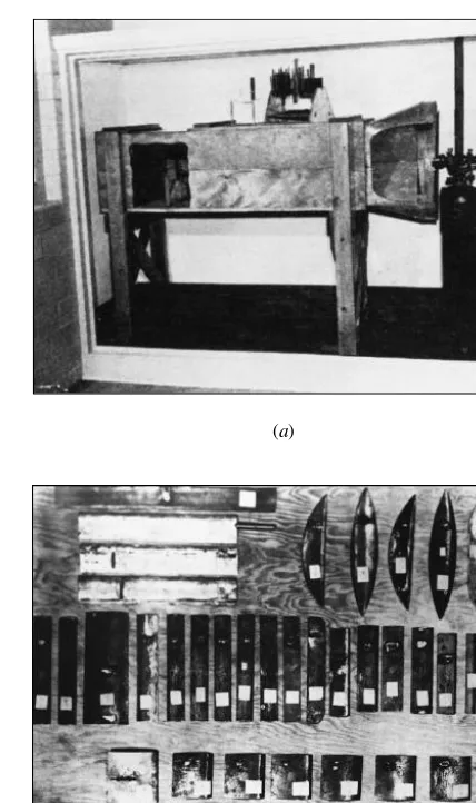
Figure 1.8 (a) Replica of the wind tunnel designed, built, and used by the Wright brothers in Dayton, Ohio, during 1901–1902. (b) Wing models tested by the Wright brothers in their wind tunnel during 1901–1902.(Photos Courtesy of the John Anderson Collection)
designs up to the present day. The importance of aerodynamics to successful manned flight goes without saying, and a major thrust of this book is to present the aerodynamic fundamentals that govern such flight.
Consider a third historical example of the importance of aerodynamics, this time as it relates to rockets and space flight. High-speed, supersonic flight had become a dominant feature of aerodynamics by the end of World War II. By this time, aerodynamicists appreciated the advantages of using slender, pointed body shapes to reduce the drag of supersonic vehicles. The more pointed and slender the body, the weaker the shock wave attached to the nose, and hence the smaller the wave drag. Consequently, the German V-2 rocket used during the last stages of World War II had a pointed nose, and all short-range rocket vehicles flown during the next decade followed suit. Then, in 1953, the first hydrogen bomb was exploded by the United States. This immediately spurred the development of long-range intercontinental ballistic missiles (ICBMs) to deliver such bombs. These vehicles were designed to fly outside the region of the earth’s atmosphere for distances of 5000 mi or more and to reenter the atmosphere at suborbital speeds of from 20,000 to 22,000 ft/s. At such high velocities, the aerodynamic heating of the reentry vehicle becomes severe, and this heating problem dominated the minds of high-speed aerodynamicists. Their first thinking was conventional—a sharp-pointed, slender reentry body. Efforts to minimize aerodynamic heating centered on the maintenance of laminar boundary layer flow on the vehicle’s surface; such laminar flow produces far less heating than turbulent flow (discussed in Chapters 15 and 19). However, nature much prefers turbulent flow, and reentry vehicles are no exception. Therefore, the pointed-nose reentry body was doomed to failure because it would burn up in the atmosphere before reaching the earth’s surface.
Figure 1.9 Energy of reentry goes into heating both the body and the air around the body.
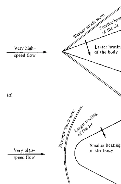
energy could be dumped into the airflow, then less would be available to be trans-ferred to the vehicle itself in the form of heating. In turn, the way to increase the heating of the airflow is to create a stronger shock wave at the nose (i.e., to use a blunt-nosed body). The contrast between slender and blunt reentry bodies is illustrated in Figure 1.10. This was a stunning conclusion—to minimize aerody-namic heating, you actually want a blunt rather than a slender body. The result was so important that it was bottled up in a secret government document. Moreover, because it was so foreign to contemporary intuition, the blunt-reentry-body con-cept was accon-cepted only gradually by the technical community. Over the next few years, additional aerodynamic analyses and experiments confirmed the validity of blunt reentry bodies. By 1955, Allen was publicly recognized for his work, receiving the Sylvanus Albert Reed Award of the Institute of the Aeronautical Sciences (now the American Institute of Aeronautics and Astronautics). Finally, in 1958, his work was made available to the public in the pioneering document NACA Report 1381 entitled “A Study of the Motion and Aerodynamic Heating of Ballistic Missiles Entering the Earth’s Atmosphere at High Supersonic Speeds.” Since Harvey Allen’s early work, all successful reentry bodies, from the first Atlas ICBM to the manned Apollo lunar capsule, have been blunt. Incidentally, Allen went on to distinguish himself in many other areas, becoming the director of the NASA Ames Research Center in 1965, and retiring in 1970. His work on the blunt reentry body is an excellent example of the importance of aerodynamics to space vehicle design.
Figure 1.10 Contrast of aerodynamic heating for slender and blunt reentry vehicles. (a) Slender reentry body. (b) Blunt reentry body.
1.2 AERODYNAMICS: CLASSIFICATION
AND PRACTICAL OBJECTIVES
A distinction between solids, liquids, and gases can be made in a simplistic sense as follows. Put a solid object inside a larger, closed container. The solid object will not change; its shape and boundaries will remain the same. Now put a liquid inside the container. The liquid will change its shape to conform to that of the container and will take on the same boundaries as the container up to the maximum depth of the liquid. Now put a gas inside the container. The gas will completely fill the container, taking on the same boundaries as the container.
The word fluidis used to denote either a liquid or a gas. A more technical distinction between a solid and a fluid can be made as follows. When a force is applied tangentially to the surface of a solid, the solid will experience afinite
stress is applied to the surface of a fluid, the fluid will experience acontinuously increasingdeformation, and the shear stress usually will be proportional to the rate of change of the deformation.
The most fundamental distinction between solids, liquids, and gases is at the atomic and molecular level. In a solid, the molecules are packed so closely together that their nuclei and electrons form a rigid geometric structure, “glued” together by powerful intermolecular forces. In a liquid, the spacing between molecules is larger, and although intermolecular forces are still strong they allow enough movement of the molecules to give the liquid its “fluidity.” In a gas, the spacing between molecules is much larger (for air at standard conditions, the spacing between molecules is, on the average, about 10 times the molecular diameter). Hence, the influence of intermolecular forces is much weaker, and the motion of the molecules occurs rather freely throughout the gas. This movement of molecules in both gases and liquids leads to similar physical characteristics, the characteristics of a fluid—quite different from those of a solid. Therefore, it makes sense to classify the study of the dynamics of both liquids and gases under the same general heading, calledfluid dynamics. On the other hand, certain differences exist between the flow of liquids and the flow of gases; also, different species of gases (say, N2, He, etc.) have different properties. Therefore, fluid dynamics is subdivided into three areas as follows:
Hydrodynamics—flow of liquids Gas dynamics—flow of gases Aerodynamics—flow of air
These areas are by no means mutually exclusive; there are many similarities and identical phenomena between them. Also, the word “aerodynamics” has taken on a popular usage that sometimes covers the other two areas. As a result, this author tends to interpret the wordaerodynamicsvery liberally, and its use throughout this book doesnotalways limit our discussions just to air.
Aerodynamics is an applied science with many practical applications in engi-neering. No matter how elegant an aerodynamic theory may be, or how mathemat-ically complex a numerical solution may be, or how sophisticated an aerodynamic experiment may be, all such efforts are usually aimed at one or more of the fol-lowing practical objectives:
1. The prediction of forces and moments on, and heat transfer to, bodies moving through a fluid (usually air). For example, we are concerned with the generation of lift, drag, and moments on airfoils, wings, fuselages, engine nacelles, and most importantly, whole airplane configurations. We want to estimate the wind force on buildings, ships, and other surface vehicles. We are concerned with the hydrodynamic forces on surface ships, submarines, and torpedoes. We need to be able to calculate the aerodynamic heating of flight vehicles ranging from the supersonic transport to a
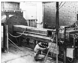
Figure 1.11 A CO2-N2gas-dynamic laser, circa 1969.(Photo Courtesy of the John Anderson Collection)
2. Determination of flows moving internally through ducts. We wish to calculate and measure the flow properties inside rocket and air-breathing jet engines and to calculate the engine thrust. We need to know the flow conditions in the test section of a wind tunnel. We must know how much fluid can flow through pipes under various conditions. A recent, very interesting application of aerodynamics is high-energy chemical and gas-dynamic lasers (see Reference 1), which are nothing more than specialized wind tunnels that can produce extremely powerful laser beams. Figure 1.11 is a photograph of an early gas-dynamic laser designed in the late 1960s.
the shock wave from the wing of a supersonic airplane impinge upon and interfere with the tail surfaces? Yet another example is the flow associated with the strong vortices trailing downstream from the wing tips of large subsonic airplanes such as the Boeing 747. What are the properties of these vortices, and how do they affect smaller aircraft which happen to fly through them?
The above is just a sample of the myriad applications of aerodynamics. One purpose of this book is to provide the reader with the technical background nec-essary to fully understand the nature of such practical aerodynamic applications.
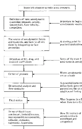
fits within the general framework of aerodynamics. For example, a road map for Chapter 1 is given in Figure 1.12. You will want to frequently refer back to these road maps as you progress through the individual chapters. When you reach the end of each chapter, look back over the road map to see where you started, where you are now, and what you learned in between.
1.4 SOME FUNDAMENTAL AERODYNAMIC
VARIABLES
A prerequisite to understanding physical science and engineering is simply learn-ing the vocabulary used to describe concepts and phenomena. Aerodynamics is no exception. Throughout this book, and throughout your working career, you will be adding to your technical vocabulary list. Let us start by defining four of the most frequently used words in aerodynamics:pressure, density, temperature,
andflow velocity.1
Consider a surface immersed in a fluid. The surface can be a real, solid surface such as the wall of a duct or the surface of a body; it can also be a free surface which we simply imagine drawn somewhere in the middle of a fluid. Also, keep in mind that the molecules of the fluid are constantly in motion.Pressureis the normal force per unit area exerted on a surface due to the time rate of change of momentum of the gas molecules impacting on (or crossing) that surface. It is important to note that even though pressure is defined as force “per unit area,” you do not need a surface that is exactly 1 ft2 or 1 m2to talk about pressure. In fact, pressure is usually defined at apointin the fluid or apointon a solid surface and can vary from one point to another. To see this more clearly, consider a point
Bin a volume of fluid. Let
dA=elemental area atB
dF=force on one side ofdAdue to pressure Then, the pressure at pointBin the fluid is defined as
p=lim
dF dA
dA→0
The pressure pis the limiting form of the force per unit area, where the area of interest has shrunk to nearly zero at the pointB.2Clearly, you can see that pressure
1A basic introduction to these quantities is given on pages 56–61 of Reference 2.
is apoint propertyand can have a different value from one point to another in the fluid.
Another important aerodynamic variable isdensity,defined as the mass per unit volume. Analogous to our discussion on pressure, the definition of density does not require an actual volume of 1 ft3or 1 m3. Rather, it is apoint property that can vary from point to point in the fluid. Again, consider a point Bin the fluid. Let
dv=elemental volume aroundB
dm =mass of fluid insidedv
Then, the density at pointBis
ρ=limdm
dv dv→0
Therefore, the densityρis the limiting form of the mass per unit volume, where the volume of interest has shrunk to nearly zero around pointB. (Note thatdvcannot achieve the value of zero for the reason discussed in the footnote concerningdA
in the definition of pressure.)
Temperaturetakes on an important role in high-speed aerodynamics (intro-duced in Chapter 7). The temperatureT of a gas is directly proportional to the average kinetic energy of the molecules of the fluid. In fact, if KE is the mean molecular kinetic energy, then temperature is given by KE= 3
2kT, wherekis the Boltzmann constant. Hence, we can qualitatively visualize a high-temperature gas as one in which the molecules and atoms are randomly rattling about at high speeds, whereas in a low-temperature gas, the random motion of the molecules is relatively slow. Temperature is also a point property, which can vary from point to point in the gas.
The principal focus of aerodynamics is fluids in motion. Hence, flow velocity is an extremely important consideration. The concept of the velocity of a fluid is slightly more subtle than that of a solid body in motion. Consider a solid object in translational motion, say, moving at 30 m/s. Then all parts of the solid are simultaneously translating at the same 30 m/s velocity. In contrast, a fluid is a “squishy” substance, and for a fluid in motion, one part of the fluid may be traveling at a different velocity from another part. Hence, we have to adopt a certain perspective, as follows. Consider the flow of air over an airfoil, as shown in Figure 1.13. Lock your eyes on a specific, infinitesimally small element of mass
and direction; hence, it is a vector quantity. This is in contrast to p,ρ, andT, which are scalar variables. The scalar magnitude ofVis frequently used and is denoted byV. Again, we emphasize that velocity is a point property and can vary from point to point in the flow.
Referring again to Figure 1.13, a moving fluid element traces out a fixed path in space. As long as the flow is steady (i.e., as long as it does not fluctuate with time), this path is called astreamlineof the flow. Drawing the streamlines of the flow field is an important way of visualizing the motion of the gas; we will frequently be sketching the streamlines of the flow about various objects. A more rigorous discussion of streamlines is given in Chapter 2.
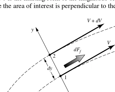
Finally, we note that friction can play a role internally in a flow. Consider two adjacent streamlinesaandbas sketched in Figure 1.14. The streamlines are an infinitesimal distance,dy, apart. At point 1 on streamlinebthe flow velocity isV;at point 2 on streamlineathe flow velocity is slightly higher,V+dV. You can imagine that streamlineais rubbing against streamlineband, due to friction, exerts a force of magnitudedFf on streamlinebacting tangentially towards the
right. Furthermore, imagine this force acting on an elemental areadA, wheredA
is perpendicular to theyaxis and tangent to the streamlinebat point 1. The local
shearstress,τ, at point 1 is
τ =lim
dF f
dA
dA→0
The shear stressτis the limiting form of the magnitude of the frictional force per unit area, where the area of interest is perpendicular to theyaxis and has shrunk
a
b dFf
V y
dy
V + dV
1 2
to nearly zero at point 1. Shear stress acts tangentially along the streamline. For the type of gases and liquids of interest in aerodynamic applications, the value of the shear stress at a point on a streamline is proportional to the spatial rate of change of velocity normal to the streamline at that point (i.e., for the flow illustrated in Figure 1.14,τ ∝dV/dy). The constant of proportionality is defined as theviscosity coefficient,μ. Hence,
τ =μd V
d y
where dV/dyis the velocity gradient. In reality,μis not really a constant; it is a function of the temperature of the fluid. We will discuss these matters in more detail in Section 1.11. From the above equation, we deduce that in regions of a flow field where the velocity gradients are small,τ is small and the influence of friction locally in the flow is small. On the other hand, in regions where the velocity gradients are large,τ is large and the influence of friction locally in the flow can be substantial.
1.4.1 Units
Two consistent sets of units will be used throughout this book, SI units (Systeme International d’Unites) and the English engineering system of units. The basic units of force, mass, length, time, and absolute temperature in these two systems are given in Table 1.1.
For example, units of pressure and shear stress are lb/ft2 or N/m2, units of density are slug/ft3 or kg/m3, and units of velocity are ft/s or m/s. When a consistent set of units is used, physical relationships are written without the need for conversion factors in the basic formulas; they are written in the pure form intended by nature. Consistent units will always be used in this book. For an extensive discussion on units and the significance of consistent units versus nonconsistent units, see pages 65–70 of Reference 2.
The SI system of units (metric units) is the standard system of units throughout most of the world today. In contrast, for more than two centuries the English engineering system (or some variant) was the primary system of units in the United States and England. This situation is changing rapidly, especially in the aerospace industry in the United States and England. Nevertheless, a familiarity with both systems of units is still important today. For example, even though most engineering work in the future will deal with the SI units, there exists a huge bulk of
Table 1.1
Force Mass Length Time Temp.
SI Units Newton kilogram meter second Kelvin
(N) (kg) (m) (s) (K)
English pounds slug feet second deg. Rankine
Engineering (lb) (ft) (s) (◦R)
make yourself comfortable in both systems.
1.5 AERODYNAMIC FORCES AND MOMENTS
At first glance, the generation of the aerodynamic force on a giant Boeing 747 may seem complex, especially in light of the complicated three-dimensional flow field over the wings, fuselage, engine nacelles, tail, etc. Similarly, the aerody-namic resistance on an automobile traveling at 55 mi/h on the highway involves a complex interaction of the body, the air, and the ground. However, in these and all other cases, the aerodynamic forces and moments on the body are due to only two basic sources:
1. Pressure distributionover the body surface 2. Shear stress distributionover the body surface
No matter how complex the body shape may be, the aerodynamic forces and moments on the body are due entirely to the above two basic sources. Theonly
mechanisms nature has for communicating a force to a body moving through a fluid are pressure and shear stress distributions on the body surface. Both pressure
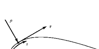
pand shear stressτ have dimensions of force per unit area (pounds per square foot or newtons per square meter). As sketched in Figure 1.15,pactsnormalto the surface, andτactstangentialto the surface. Shear stress is due to the “tugging action” on the surface, which is caused by friction between the body and the air (and is studied in great detail in Chapters 15 to 20).
The net effect of the pandτ distributions integrated over the complete body surface is a resultant aerodynamic forceRand momentMon the body, as sketched in Figure 1.16. In turn, the resultantRcan be split into components, two sets of
Figure 1.16 Resultant aerodynamic force and moment on the body.
Figure 1.17 Resultant aerodynamic force and the components into which it splits.
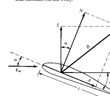
which are shown in Figure 1.17. In Figure 1.17,V∞is therelative wind,defined as the flow velocity far ahead of the body. The flow far away from the body is called the freestream, and hence V∞ is also called the freestream velocity. In Figure 1.17, by definition,
L ≡lift≡component ofRperpendicular toV∞
D ≡drag≡component ofRparallel toV∞
The chordcis the linear distance from the leading edge to the trailing edge of the body. Sometimes,Ris split into components perpendicular and parallel to the chord, as also shown in Figure 1.17. By definition,
N ≡normal force≡component ofRperpendicular toc
A≡axial force≡component ofRparallel toc
The angle of attack α is defined as the angle between cand V∞. Hence,α is also the angle betweenLandN and betweenDandA. The geometrical relation between these two sets of components is, from Figure 1.17,
L= Ncosα−Asinα (1.1)
Figure 1.18 Nomenclature for the integration of pressure and shear stress distributions over a two-dimensional body surface.
Let us examine in more detail the integration of the pressure and shear stress distributions to obtain the aerodynamic forces and moments. Consider the two-dimensional body sketched in Figure 1.18. The chord line is drawn horizontally, and hence the relative wind is inclined relative to the horizontal by the angle of attackα. Anx ycoordinate system is oriented parallel and perpendicular, respec-tively, to the chord. The distance from the leading edge measured along the body surface to an arbitrary pointAon the upper surface issu; similarly, the distance
to an arbitrary point Bon the lower surface issl. The pressure and shear stress
on the upper surface are denoted bypuandτu, bothpuandτuare functions ofsu.
Similarly, pl andτl are the corresponding quantities on the lower surface and
are functions ofsl. At a given point, the pressure is normal to the surface and
is oriented at an angleθ relative to the perpendicular; shear stress is tangential to the surface and is oriented at the same angleθ relative to the horizontal. In Figure 1.18, the sign convention forθis positive when measuredclockwisefrom the vertical line to the direction ofpand from the horizontal line to the direction ofτ. In Figure 1.18, all thetas are shown in their positive direction. Now con-sider the two-dimensional shape in Figure 1.18 as a cross section of an infinitely long cylinder of uniform section. A unit span of such a cylinder is shown in Figure 1.19. Consider an elemental surface areadSof this cylinder, wheredS=
(ds)(1) as shown by the shaded area in Figure 1.19. We are interested in the contribution to the total normal forceN′and the total axial force A′due to the
pressure and shear stress on the elemental areadS. The primes on N′ and A′
Figure 1.19 Aerodynamic force on an element of the body surface.
upperbody surface are
d Nu′ = −pudsucosθ−τudsusinθ (1.3)
dA′u = −pudsusinθ+τudsucosθ (1.4)
On thelowerbody surface, we have
d Nl′= pldslcosθ−τldslsinθ (1.5)
dA′l = pldslsinθ+τldslcosθ (1.6)
In Equations (1.3) to (1.6), the positive directions ofN′andA′are those shown in
Figure 1.17. In these equations, the positive clockwise convention forθmust be followed. For example, consider again Figure 1.18. Near the leading edge of the body, where the slope of the upper body surface is positive,τis inclined upward, and hence it gives a positive contribution toN′. For an upward inclinedτ,θwould
be counterclockwise, hence negative. Therefore, in Equation (1.3), sinθ would be negative, making the shear stress term (the last term) a positive value, as it should be in this instance. Hence, Equations (1.3) to (1.6) hold in general (for both the forward and rearward portions of the body) as long as the above sign convention forθ is consistently applied.
The total normal and axial forcesper unit spanare obtained by integrating Equations (1.3) to (1.6) from the leading edge (LE) to the trailing edge (TE):
N′= −
TE LE
(pucosθ+τusinθ )dsu+ TE
LE
(plcosθ−τlsinθ )dsl (1.7)
A′=
TE LE
(−pusinθ+τucosθ )dsu+ TE
LE
In turn, the total lift and drag per unit span can be obtained by inserting Equa-tions (1.7) and (1.8) into (1.1) and (1.2); note that EquaEqua-tions (1.1) and (1.2) hold for forces on an arbitrarily shaped body (unprimed) and for the forces per unit span (primed).
The aerodynamic moment exerted on the body depends on the point about which moments are taken. Consider moments taken about the leading edge. By convention, moments that tend to increaseα(pitch up) are positive, and moments that tend to decreaseα(pitch down) are negative. This convention is illustrated in Figure 1.20. Returning again to Figures 1.18 and 1.19, the moment per unit span about the leading edge due topandτon the elemental areadSon the upper surface is
d Mu′ =(pucosθ+τusinθ )x dsu+(−pusinθ+τucosθ )y dsu (1.9)
On the bottom surface,
d Ml′=(−plcosθ+τlsinθ )x dsl+(plsinθ+τlcosθ )y dsl (1.10)
In Equations (1.9) and (1.10), note that the same sign convention forθ applies as before and thatyis a positive number above the chord and a negative number below the chord. Integrating Equations (1.9) and (1.10) from the leading to the trailing edges, we obtain for the moment about the leading edge per unit span
MLE′ =
TE LE
[(pucosθ+τusinθ )x−(pusinθ−τucosθ )y]dsu
(1.11)
+ TE
LE
[(−plcosθ+τlsinθ )x+(plsinθ+τlcosθ )y]dsl
In Equations (1.7), (1.8), and (1.11), θ, x, and y are known functions ofs
for a given body shape. Hence, if pu, pl,τu, andτl are known as functions ofs
(from theory or experiment), the integrals in these equations can be evaluated. Clearly, Equations (1.7), (1.8), and (1.11) demonstrate the principle stated earlier, namely,the sources of the aerodynamic lift, drag, and moments on a body are the pressure and shear stress distributions integrated over the body.A major goal of theoretical aerodynamics is to calculatep(s)andτ (s)for a given body shape and freestream conditions, thus yielding the aerodynamic forces and moments via Equations (1.7), (1.8), and (1.11).
As our discussions of aerodynamics progress, it will become clear that there are quantities of an even more fundamental nature than the aerodynamic forces and moments themselves. These aredimensionless force and moment coefficients,
the freestream, far ahead of the body. We define a dimensional quantity called the freestreamdynamic pressureas
Dynamic pressure: q∞≡ 12ρ∞V2
∞
The dynamic pressure has the units of pressure (i.e., pounds per square foot or newtons per square meter). In addition, let S be a reference area andl be a reference length. The dimensionless force and moment coefficients are defined as follows:
Lift coefficient: CL ≡
L q∞S
Drag coefficient: CD≡
D q∞S
Normal force coefficient: CN ≡
N q∞S
Axial force coefficient: CA ≡
A q∞S
Moment coefficient: CM ≡
M q∞Sl
In the above coefficients, the reference areaSand reference lengthl are chosen to pertain to the given geometric body shape; for different shapes,Sandlmay be different things. For example, for an airplane wing,Sis the planform area, andl
is the mean chord length, as illustrated in Figure 1.21a. However, for a sphere,
S is the cross-sectional area, andl is the diameter, as shown in Figure 1.21b.