arXiv:1011.2017v1 [math.CV] 9 Nov 2010
parameters
C. D´ıaz Mendoza Univ. de La Laguna, Spain
R. Orive
Univ. de La Laguna, Spain [email protected]
November 10, 2010
Abstract
We study the asymptotic zero distribution of the rescaled Laguerre polynomials, L(αn)
n (nz), with the parameter αn varying in such a way that lim n→∞α
n/n = −1. The
connection with the so-called Szeg¨o curve will be showed.
1
Introduction
The definition and many properties of the Laguerre polynomials L(nα) can be found in Ch. V
of Szeg˝o’s classic memoir [21]. Given explicitly by
L(nα)(z) =
n
X
k=0
n+α n−k
(−z)k
k! , (1.1)
or, equivalently, by the well-known Rodrigues formula
L(nα)(z) = (−1)
n
n! z −αez
d dz
n
zn+αe−z , (1.2)
they can be considered for arbitrary values of the parameterα∈C. In particular, (1.1) shows that each L(nα) depends analytically on α and no degree reduction occurs: degL(nα) = n for
all α∈C.
Forα >−1 it is well-known the orthogonality of L(nα)(x) on [0,+∞) with respect to the
weight functionxαe−x; in particular, all their zeros are simple and belong to [0,+∞). In the
general case, α ∈ C, L(nα)(z) may have complex zeros; the only multiple zero can appear at
z= 0, which occurs if and only if α∈ {−1,−2, . . . ,−n}. In this case we have
L(n−k)(z) = (−z)k(n−k)!
n! L
(k)
n−k(z), (1.3)
which shows that z= 0 is a zero of multiplicity k forL(n−k)(z).
In a series of papers ([7], [8] and [12]), asymptotics for rescaled Laguerre polynomials
L(αn)
n (nz) were analyzed, under the assumption that limn→∞αn/n = A ∈ R. In [12] the
au-thors obtained the weak zero asymptotics for the case where A <−1, by means of classical (logarithmic) potential theory. To this end, it played a key role a full set of non-hermitian orthogonality relations satisfied by Laguerre polynomials in a class of open contours in C. Unfortunately, this analysis could not be extended to the other cases, since for this approach it is essential the connectedness of the complement to the support of the asymptotic distribu-tion of zeros (see e.g. [5] and [18]). However, the authors formulated in [12] a conjecture for the case −1< A <0, which was proved in some cases and refused in others in [8], by means of the Riemann-Hilbert approach (which has been previously used by the same authors in [7] to obtain strong asymptotics in the case A < −1). A similar study for Jacobi polynomials with varying nonstandard parameters has been carried out in [9], [11] and [13].
Jacobi or Laguerre polynomials with real parameters (and in general, depending on the degree n) appear naturally as polynomial solutions of hypergeometric differential equations, or in the expressions of the wave functions of many classical systems in quantum mechanics (see e.g. [2]).
In [12], the authors also formulated a conjecture for the caseA=−1, but up to now this problem has remained open. Observe that, by (1.3), when k=nwe have:
L(n−n)(z) = (−1)n 1
n!z
n.
There is another particular situation corresponding to the case A =−1 which is very well-known in the literature: whenαn=−n−1, we have:
L(n−n−1)(z) = (−1)n
n
X
k=0
zk k! ,
and thus, in this case the Laguerre polynomials agree (up to a possible sign) with the partial sums of the exponential series. In a seminal paper, G. Szeg˝o [20] showed that the zeros of the
rescaled partial sums of the exponential series,
n
X
k=0
(nz)k
k! = (−1)
nL(−n−1)
n (nz), approach
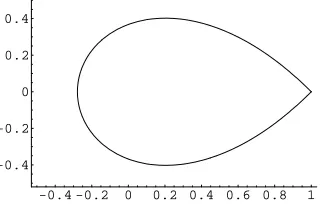
the so-called the Szeg˝o curve:
means of the Riemann-Hilbert analysis. Also, in [3], the authors studied the asymptotics of orthogonal polynomials with respect to modified Laguerre weights of the type
z−n+νe−N z(z−1)2b,
where n, N → ∞ withN/n→1 andν is a fixed number in R\N.
-0.4 -0.2 0 0.2 0.4 0.6 0.8 1 -0.4
-0.2 0 0.2 0.4
Figure 1: The Szeg˝o curve.
In this paper, the weak zero asymptotics of rescaled Laguerre polynomials L(αn)
n (nz),
with lim
n→∞αn/n = −1 will be analyzed. For it, we will prove that such rescaled Laguerre polynomials are asymptotically extremal on certain well defined curves in the complex plane. The outline of the paper is as follows. In sect 2, the main result about the weak zero asymptotics of the rescaled Laguerre polynomials is announced, and in sect. 3, some basic facts on potential theory and asymptotically extremal polynomials are recalled. Finally, the proofs are given in sect. 4.
2
Main Result
Along with the Szeg¨o curve (1.4), we need to introduce the family of level curves:
Γr = z∈C,
ze1−z=e−r,|z| ≤1 ,0≤r <+∞, (2.1)
while for r =∞ we take Γ∞={0}. Observe that Γ0 = Γ, the Szeg˝o curve. We consider the
usual counterclockwise orientation. All the level curves Γr (0≤r <+∞) are closed contours
such that {0} ⊂ Int(Γr) and Γr′ ⊂Int(Γr), for r′ > r. On the sequel, the interior of Γr will
be denoted byGr. Associated with this family of curves, consider for 0≤r <+∞the family
of measures:
dµr(z) =
1 2πi
1−z
z dz , z∈Γr, (2.2)
Let us recall the definition of balayage (or sweeping out) of a measure (see e.g. [16]). Given an open set Ω with compact boundary ∂Ω and a positive measure σ with compact support in Ω, there exists a positive measure bσ, supported in∂Ω, such thatkσk=kbσkand
Vbσ(z)−Vσ(z) = const, qu.e.z /∈Ω, (2.3)
where const = 0 when Ω is a bounded set, and a property is said to be satisfied for “quasi-every” (qu.e.) zin a certain set, if it holds except for a possible subset of zero (logarithmic) capacity. Then, bσ is said to be the balayage ofσ from Ω onto ∂Ω.
Now, we have the following:
Lemma 1 The a priori complex measure (2.2) is a unit positive measure in Γr (2.1), for
0 ≤ r < +∞ . Moreover, µr is the balayage of δ0 from Gr onto Γr, where δ0 denotes the
Dirac Delta at z= 0.
Now, for each n ∈ N, consider the “pathological” subset of negative integers Sn =
{−n,−(n−1), . . . ,−2,−1}.Hereafter, suppose that αn∈/Sn.
Finally, denote by dist(αn,Sn) > 0 the minimal distance between αn and the set Sn.
Theorem 1 Consider a sequence of rescaled Laguerre polynomials{L(αn)
n (nz)}n∈N, such that
lim
n→∞
αn
n = −1 and
lim
n→∞[dist(αn,Sn)]
1/n = e−r, (2.4)
for some r ≥0.Then, the contracted zeros of Laguerre polynomials asymptotically follow the measure dµr in (2.2)on the curve Γr (2.1). For r= +∞, the limit measure is dµ∞ = δ0.
Remark 1 The results above also hold when dealing with infinite subsequences{L(αn)
n (nz)}n∈Λ, Λ⊂
N.
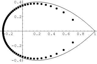
Remark 2 Observe that the caser= 0 in Theorem 1 is generic, because it takes place when
parameters αn do not approach, or, at least, do not approach exponentially fast, the set of
integers Sn (see Figure 2). On the other hand, when r > 0 and, so, parameters approach the set of integers Sn exponentially fast, the Szeg˝o curve Γ is replaced by a level curve Γr which surrounds z = 0 and is strictly contained in the interior of Γ (see Figure 3). Finally, when r =∞, i.e., when parameters approach the set Sn faster than exponentially, the limit measure reduces to a Dirac mass at z= 0.
Remark 3 The weak asymptotics in the caseA=−1,characterized for the set of measures
-0.2 0.2 0.4 0.6 0.8 1
-0.4 -0.2 0.2 0.4
Figure 2: The Szeg˝o curve and the zeros of L(60−60.1)(60z).
-0.2 0.2 0.4 0.6 0.8 1
-0.4 -0.2 0.2 0.4
Figure 3: Zeros of L(60−60+10−5)(60z) and the curve Γr, forr= 121 ln 10.
the following full set of non-hermitian orthogonality relations for the Laguerre polynomials with parameters α∈C was used:
Z
Σ
L(nα)(z)zkzαe−zdz = 0, k= 0, . . . , n−1,
where Σ is any unbounded contour in C\[0,∞), connecting +∞+iy and +∞ −iy , for some y >0,and the branch in zα is taken with the cut along the positive real axis (see [7, Lemma 2.1]). In [12] this full set of orthogonality relations allowed to apply seminal results by H. Stahl [18] and A. Gonchar and E. A. Rakhmanov [5] on the asymptotic behavior of complex orthogonal polynomials. Indeed, it was proved that zeros of the rescaled Laguerre polynomials accumulate on a closed contour C in C\[0,∞) which is “symmetric” (in the “Stahl’s sense”, see [17]-[18]) with respect to the external fieldϕ(z) = 12(−Alog|z|+ Rez),
and that they asymptotically follow the equilibrium distribution on C in presence of the external field ϕ. In the proof of the main result in this paper, it will be showed that the zeros of the rescaled Laguerre polynomials in the present case also asymptotically follow the equilibrium distribution of Γr in presence of the external field ϕ above (for A = −1 ), Γr
3
On asymptotically extremal polynomials
Throughout this section, some topics in potential theory which are needed for the proof of our main result will be recalled. For more details the reader can consult the monography [16].
First, let us precise the notion of admissible weights.
Definition 1 Given a closed set Σ ⊂ C, we say that a function ω : Σ −→ [0,∞) is an admissible weight on Σ if the following conditions are satisfied (see [16, Def.I.1.1]):
(a) ω is upper semi-continuous;
(b) the set {z∈Σ :ω(z)>0}has positive (logarithmic) capacity; (c) if Σ is unbounded, then lim
|z|→∞, z∈Σ|z|ω(z) = 0.
Given such an admissible weightω in the closed set Σ, and settingϕ(z) =−logω(z), we know (see e.g. [16, Ch.I]) that there exists a unique measureµω, with (compact) support in
Σ, for which the infimum of the weighted (logarithmic) energy
Iω(µ) = −
Z Z
log|z−x|dµ(z)dµ(x) + 2 Z
ϕ(x)dµ(x)
is attained. Moreover, setting Fω =Iω(µω)−
Z
ϕdµω, which is called the modified Robin
constant, we have the following property, which uniquely characterizes the extremal measure
µω:
Vµω
(z) +ϕ(z) (
= Fω, qu.e. z∈suppµω,
≥ Fω, qu.e. z∈Σ,
where for a measure σ,Vσ denotes its logarithmic potential, that is,
Vσ(z) = −
Z
log|z−x|dσ(x).
Now, let Σ be a closed set and ω an admissible weight on Σ. Then, a sequence of monic polynomials {pn}n∈N is said to be asymptotically extremal with respect to the weightω if it
holds (see [16]):
lim
n→∞kω
np
nk1Σ/n = exp(−Fω), (3.1)
where, as usual,k·kK denotes the sup-norm in the setK .The study of weighted polynomials
of the form ω(z)nPn(z) has applications to many problems in approximation theory (see e.g.
the monographies [16] and [22]). It is well known that if for each n ∈ N, Tω
(weighted) Chebyshev polynomial with respect to the weight ωn, that is, if it is the (unique) monic polynomial of degree nfor which the infimum
tωn = inf{kωnPkΣ, P(z) =zn+. . .}
is attained, then the sequence {Tnω}satisfies the asymptotic behavior given in (3.1) (see [16, Ch.III]).
Under mild conditions on the weight ω, in [16, Ch.III] it is shown that the zeros of such sequences of polynomials asymptotically follow the equilibrium measure µω, in the sense of
the weak-* convergence. Indeed, we have the following result (see [16, Th.III.4.1] or the previous paper [14]):
Theorem 2 Let ω be an admissible weight such that the support of the corresponding equi-librium measure µω, Sω, has zero Lebesgue planar measure. Let {pn}n∈N be a sequence of monic polynomials of respective degrees n= 1,2, . . . satisfying:
lim
n→∞kω
np
nk1S/nω = exp(−Fω), (3.2)
where Fω denotes the modified (by the external field ϕ=−lnω) Robin constant. Then, the
following statements are equivalent:
(a) ν(pn)−→µω in the weak-* sense, where ν(pn) denotes the unit zero counting measure
associated to pn, that is, dν(pn) =
1
n
X
pn(ζ)=0
δζ.
(b) For each bounded component R of C\Sω and each infinite sequence N⊂N, there exist
z0∈R and N1⊂N such that
lim
n→∞,n∈N1
|pn(z0)|1/n = exp(−Vµω(z0)). (3.3)
Remark 4 In [4, Theorem 5], condition (3.2) is replaced by the weaker condition:
lim sup
n→∞ ω(z)|pn(z)|
1/n ≤ exp(−F
ω), qu.e.z∈Sω. (3.4)
Remark 5 It is clear that the balayage of a measure (see (2.3)) is a very particular case
of equilibrium measure in an external field. Since Lemma 1 says that measure µr is the
balayage of δ0 from Gr onto its boundary Γr,it means that
Vµr
(z) = −log|z|, z∈Γr. (3.5)
Taking into account the expression of Γr,(3.5) implies both
Vµr
and
For the proof of Theorem 1, taking into account Theorem 2, it will be proved that the rescaled Laguerre polynomials are asymptotically extremal with respect to the weight ω =
e−ϕ in the compact set given by the closed contour Γr (using (3.4)), along with the fact that
they satisfy the local behavior (3.3).
4
Proofs
4.1 Proof of Lemma 1
Take into account that the level curves Γr, for 0 ≤ r < ∞, given by (2.1) are, in fact,
trajectories of the quadratic differential (see e.g. [19])
−(z−1)
Expression (4.1) shows that (2.2) is real-valued in Γr and does not change its sign. Moreover,
by a straightforward application of the Cauchy theorem, we have that
µr(Γr) =
Thus, from (2.2), we have:
dµr(z) = measure at z = 0 with respect to the domain Gr. But this fact implies that (2.2) is the
4.2 Proof of Theorem 1
In Remark 5, it was shown thatµr is also the equilibrium measure in Γr in the external field
ϕ (3.8).
Moreover, (3.7) shows that the corresponding modified Robin constant is given by:
Fω =
r+ 1
2 . (4.2)
On the other hand, the function g(z) = Vµr
(z) + Rez is harmonic in Gr and, by (3.6),
g(z) ≡ r+ 1, z∈Γr.Then, it yields thatg(z) ≡ r+ 1, z∈Gr.In particular,
Vµr
(0) = r+ 1. (4.3)
From (4.2), in order to prove (3.4) we need to show that
lim sup
n→∞ ω(z)|pn(z)|
1/n ≤ e−r+1
2 , qu.e.z∈Γr,
for the monic polynomial pn(z) = Lb(αn)
n (nz) and the weight ω(z) = e−ϕ(z), which taking
into account the expression of Γr, is equivalent to prove:
lim sup
n→∞
e−Rez|pn(z)|1/n ≤ e−(r+1), qu.e.z∈Γr. (4.4)
Now, since by (1.1) L(αn)
n (nz) = lαnnzn+. . ., with
lαn
n = (−1)n
nn
n! , (4.5)
we have that (4.4) is equivalent to
lim sup
n→∞ e
−Rez|L(αn)
n (nz)|1/n ≤ e−r, qu.e.z∈Γr. (4.6)
In addition, we should prove that there exists a point z0 ∈ Gr for which (3.3) is attained.
Thus, choosing z0 = 0, and taking into account (4.3), it is enough to show that
lim
n→∞|pn(0)|
1/n
= e−(r+1),
or what is the same, by (4.5),
lim
n→∞ L(αn)
n (0)
1/n = e−r. (4.7)
4.2.1 Proof of (4.7)
Take into account that by (1.1),
L(αn)
and, therefore, to prove (4.7) it should be satisfied:
lim
and taking into account that 2k−1
from which it yields
In order to prove (4.6), the following integral representation will be used (see [1, formula (6.2.22)]):
where β > α and the path of integration is any simple smooth path connecting x ∈C with +∞.Thus, setting β=−kn and α=αn in (4.10) and taking into account (4.9), we have:
or what is the same, after some calculations,
On the other hand, taking into account the Rodrigues formula (1.2), (4.12) yields:
semiaxis. Now, using the freedom in the choice of the path of integration, it will consists of two arcs: the first goes from x to x0 through the curve Γr (by the shortest way), and the
corresponding integral will be denoted by Gn(x); the second goes from x0 to ∞ along the
positive real semiaxis, and we will denote this integral by Hn(x). Thus, Fn(x) = Gn(x) +
Since the path of integration is a smooth recitifiable Jordan arc (even for the case when
r = 0,since the path is entirely contained in the upper, or lower, half of Γ0 = Γ ), we have
Then, by classical mean value
where lim
Proceeding analogously as above, it holds
|Gn(x)| ≤ An
and thus, by applying the Cauchy integral formula in an arbitrarilly small circle around t ,
we have for tin the segment of curve Γr connectingx to x0,
forǫ >0 arbitrarily small. Hence,
|Gn(x)| ≤ An(n−kn)!ǫ−n+kn
fore, by (4.14)-(4.17), it yields
lim sup
n→∞ (|∆nGn(x)|)
1/n ≤ e−r, x∈Γ
r\ {x0}, (4.18)
Now, we are concerned with Hn(x).As above, suppose first that kn=n , and thus,
where now the path of integration is contained in the positive real semiaxis. Then, we have
Hn(x) = en
and integrating by parts, it yields
Now, applying again the Cauchy integral formula for t∈[x0,∞)⊂R+,it holds:
[(φ(t))n](l) ≤ l!ǫ−le2ǫnφ(t+ε)n, (4.22)
for arbitrarily small ǫ >0.
Then, taking into account (4.21)-(4.22) and setting
Dn = (n−kn−1)!ǫ−n+kn+1e2ǫn|x0−x|δn−1,
Finally, we can bound the integral above as in (4.19), which yields
|Hn(x)| ≤ Dn (φ(x0+ε)n + (1−δn)Mf−1e−1
Now, from (4.20), (4.23) and (4.24), it follows
lim sup
n→∞ (|∆nHn(x)|)
1/n
≤ e−r, x∈Γr\ {x0}, (4.25)
after taking limits when ε→0+,if necessary. Thus, from (4.18) and (4.25), it yields
lim sup
n→∞ (|∆nFn(x)|)
1/n ≤ e−r, x∈Γ
It only remains to consider the limit caser=∞,which occurs when lim
n→∞[dist(αn,
Sn)]1/n = 0.
Having in mind the method above, it is not hard to see that in this case, we have that
lim sup
n→∞ e
−Rex|L(αn)
n (nx)|1/n ≤ e−s, x∈Γs\ {x0(s)}, (4.26)
for any s > 0. Thus, applying [4, Theorem 5], (4.26) implies that suppµ∞ ⊂ Gs, for any
s >0. Since \
s>0
Gs ={0},the conclusion easily follows.
Acknowledgements
R.O. thanks Professors A. B. J. Kuijlaars, A. Mart´ınez Finkelshtein and H. Stahl for useful discussions.
References
[1] G. E. Andrews, R. Askey and R. Roy,Special functions, Encyclopedia of Mathe-matics and its Applications 71, Cambridge University Press, Cambridge, 1999.
[2] V. G. Bagrov and D. M. Gitman, Exact Solutions of Relativistic Wave Equations, Kluwer Academic Publ., Dordrecht, 1990.
[3] D. Dai and A. B. J. Kuijlaars, Painlev´e IV asymptotics for orthogonal polynomials with respect to a modified Laguerre weight, Stud. Appl. Math.122, no. 1 (2009), 29–83.
[4] W. Gautschi and A. B. J. Kuijlaars, Zeros and critical points of Sobolev Orthogonal Polynomials, J. Approx. Theory91 (1997), 117–137.
[5] A. A. Gonchar and E. A. Rakhmanov, Equilibrium distributions and the rate of rational approximation of analytic functions,Mat. USSR Sbornik62 (2) (1989), 305–348.
[6] T. Kriecherbauer, A. B. J. Kuijlaars, K.D.T-R McLaughlin and P.D. Miller, Locating the zeros of partial sums of exp(z) with Riemann-Hilbert methods, to appear in Contemporary Mathematics, in ”Integrable Systems and Random Matrices: in honor of Percy Deift”, Contemporary Mathematics 458, Amer. Math. Soc., Providence R.I. 2008, pp. 183–196.
[8] A. B. J. Kuijlaars and K. T-R McLaughlin, Asymptotic zero behavior of Laguerre polynomials with negative parameter, Constr. Approx.20 (2004), 497–523.
[9] A. B. J. Kuijlaars and A. Mart´ınez-Finkelshtein, Strong asymptotics for Jacobi polynomials with varying nonstandard parameters, J. d’Analyse Math. 94 (2004), 195– 234.
[10] N. S. Landkof,Foundations of Modern Potential Theory, Springer-Verlag, Berlin, 1972.
[11] A. Mart´ınez-Finkelshtein, P. Mart´ınez-Gonz´alez and R. Orive, Zeros of Ja-cobi polynomials with varying non-classical parameters, inSpecial functions(Hong Kong, 1999), World Sci. Publishing, River Edge, NJ, 2000, pp. 98–113.
[12] A. Mart´ınez-Finkelshtein, P. Mart´ınez-Gonz´alez and R. Orive, On asymp-totic zero distribution of Laguerre and generalized Bessel polynomials with varying pa-rameters, J. Comput. Appl. Math.133 (2001), 477–487.
[13] A. Mart´ınez-Finkelshtein and R. Orive, Riemann-Hilbert analysis for Jacobi poly-nomials orthogonal on a single contour, J. Approx. Theory 134 (2005), 137–170.
[14] H. N. Mhaskar and E. Saff, The distribution of zeros of asymptotically extremal polynomials,J. Approx. Theory 65 (1991), 279–300.
[15] I. Pritsker and R. Varga, The Szeg¨o curve, zero distribution and weighted approx-imation,Trans. Amer. Math. Soc. 349, 4085–4105.
[16] E.B. Saff and V. Totik,Logarithmic Potentials with External Fields, volume 316 of
Grundlehren der Mathematischen Wissenschaften (Springer-Verlag, Berlin, 1997).
[17] H. Stahl, Extremal domains associated with an analytic function. I, II,Complex Vari-ables Theory Appl.4 (4) (1985) 311-324, 325-338.
[18] H. Stahl, Orthogonal polynomials with complex-valued weight function I and II, Con-str. Approx.2 (1986), 225–240, 241–251.
[19] K. Strebel,Quadratic Differentials, Springer, Berlin, 1984.
[20] G. Szeg˝o, ¨Uber eine Eigenschaft der Exponentialreihe, Sitzungsber. Berl. Math. Ges.
23 (1924), 50–64.
[21] G. Szeg˝o,Orthogonal Polynomials, volume 23 ofAmer. Math. Soc. Colloq. Publ.(Amer. Math. Soc., Providence, fourth edition, 1975).