A Language for Spatial Data Manipulation

03JEI0000 1726-2135/1684-8799  2003 ISEIS www.iseis.org/jei.htm Journal of Environmental Informatics

A Language for Spatial Data Manipulation

B. Howe1*, D. Maier1, A. Baptista2

1

Department of Computer Science and Engineering, OGI School of Science and Engineering at Oregon Health and Science University, 20000 NW Walker Road, Beaverton, OR 97006

2

Department of Environmental and Biomolecular Systems, OGI School of Science and Engineering at Oregon Health and Science University, 20000 NW Walker Road, Beaverton, OR 97006

ABSTRACT. Environmental Observation and Forecasting Systems (EOFS) create new opportunities and challenges for generation and use of environmental data products. The number and diversity of these data products, however, has been artificially constrained by the lack of a simple descriptive language for expressing them. Data products that can be described simply in English take pages of obtuse scripts to generate. The scripts obfuscate the original intent of the data product, making it difficult for users and scientists to understand the overall product catalog. The problem is exacerbated by the evolution of modern EOFS into data product “factories” subject to reliability requirements and daily production schedules. New products must be developed and assimilated into the product suite as quickly as they are imagined. Reliability must be maintained despite changing hardware, changing software, changing file formats, and changing staff. We present a language for naturally expressing data product recipes over structured and unstructured computational grids of arbitrary dimension. Informed by relational database theory, we have defined a simple data model and a handful of operators that can be composed to express complex visualizations, plots, and transformations of gridded datasets. The language provides a medium for design, discussion, and development of new data products without commitment to particular data structures or algorithms. In this paper, we provide a formal description of the language and several examples of its use to express and analyze data products. The context of our research is the CORIE system, an EOFS supporting the study of the Columbia River Estuary.

Keywords: Columbia River, database, data model, data product, estuarine, grid, visualization

1. Introduction

Scientific data processing consists of two distinct steps: dataset retrieval and dataset analysis. These tasks are not difficult when the amount of data is modest: Datasets can be retrieved by browsing the filesystem, analysis routines can be invoked manually, and the resulting data products can be returned to the filesystem and organized in an ad hoc manner. However, as the amount of data grows, a scalable and comprehensive set of policies, embodied by some form of data management system, is required. Existing database technology supports dataset retrieval, but dataset analysis must be performed using specialized programs. These specialized programs, however, are generally designed for analyzing one dataset at a time, and are difficult to incorporate into large-scale data management systems. Scientists need to apply the same program to hundreds or thousands of datasets simultaneously, compose programs in non-trivial ways, and author new programs at a rapid rate. The focus of our work has been to understand the fundamental manipulations per-formed by such programs, and propose a simple language that can express such manipulations.

Scientific datasets are often characterized by the topo-logical structure, or grid, over which they are defined. For example, a timeseries is defined over a 1-dimensional grid,

* Corresponding author: bill@cse.ogi.edu

while the solution to a partial differential equation using a finite element method might be defined over a 3-dimensional grid. Grids therefore seem an appropriate concept on which to base a scientific data model. Indeed, others have observed that grid patterns appear frequently in a wide range of domains (Berti, 2000; Moran, 2001; Kurc et al., 2001; Schroeder et al., 2000; OpenDX, 2002; Treinish, 1996; Haber

et al., 1991). What has not been previously observed is the

existence of simple patterns in grid manipulations; that much of the extensive library code provided with scientific visualization systems, for example, can be cast in terms of just a few fundamental operators?

using an Eulerian-Lagrangian finite element method. The horizontal grid is parallel to the water’s surface extends from the Baja peninsula up to Alaska, though the Columbia River Estuary and the ocean waters around the mouth of the river have the greatest concentration of grid elements. Using a vertical grid to partition the depth of the river, a 3-dimensional grid can be generated. Time steps add a fourth dimension.

Longview Upstream limit

Bonneville Dam

Willamette Falls

Figure 1. The CORIE grid, extending from the Baja peninsula to Alaska, to model the influence of the Columbia River.

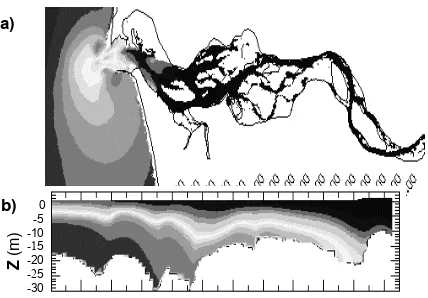
Data defined over this grid include the physical charac-teristics of the flowing water: velocity, temperature, salinity, elevation. Three classes of data products in the product suite are contour plots projected onto the horizontal grid, contour plots projected onto some vertical grid, and timeseries plots. Horizontal contour plots take a “slice” through the grid in the xy plane, perhaps aggregating over the vertical dimension. Figure 2a shows a horizontal slice at a depth of three meters. Vertical contour plots such the one in Figure 2b also “slice” through the grid, but in the vertical direction. In this case, the unstructured horizontal grid in Figure 1 does not appear in the output; rather a new grid is formed from user-selected points in the xy plane extended in the vertical dimension. Figure 2b was taken from points along a channel near the mouth of the river. Timeseries data products are standard 2-dimensional graphs with one or more variables plotted against time.

1.1. Challenges

The existing CORIE data product pipeline consists of C programs controlled by Perl scripts. A fixed set of data products can be reliably generated using this approach, but new data products are difficult to define and incorporate into the product suite. In fact, design, construction, and assimilation of new data products are currently intractable for those not intimately familiar with CORIE file formats and processing environments; these tasks are certainly beyond the reach of non-technical consumers of CORIE data. Our work takes steps toward lowering development time for both expert users and non-expert users.

a)

b) ₀

-5

-10

-15

-20

-25

-30

Z

(m)

b)

Figure 2.Two data products in the CORIE system: (a) Horizontal slice showing salinity in the estuary; (b) Vertical slice along a channel of the same data.

Since many data products are visualizations, our first ap-proach was to investigate mature visualization libraries to replace or augment our custom codes. IBM's Data Explorer (DX) (OpenDX, 2002) and the Visualization Toolkit (VTK) (Schroeder et al., 1996) are free software libraries implementing efficient visualization algorithms in an organized library. We gave these libraries most of our attention since they are freely available and widely used. However, other tools such as Geographic Information Systems (GIS) and general scientific data management platforms are relevant and are discussed in Section 6.

DX and VTK support a rich set of visualization opera-tions, but their use did not significantly lower development time. New data products were still difficult to define and assimilate. Minor changes in the conceptual data product specification required major changes to the code. Data products that were easy to describe in English still required rather obtuse programming constructs. Even experienced users of VTK had trouble applying their knowledge to the CORIE datasets. Prior to implementation, we described data products in English using natural concepts such as a “horizontal or vertical slice” and the “maximum over depth”. Unfortunately, these concepts did not always have analogous operations in the library. We significant time translating our concepts into the “language” of VTK and DX. Specifically, the following concepts proved useful but were poorly supported by both libraries:

Cross Product Grids. We found that the notion of cross product is able to express many common grid ma-nipulations: constructing higher dimensional grids, repeating data values, and describing the relationship between two grids.

Shared Grids. Many datasets tend to be defined over the same grid, with each dataset corresponding to a variation in simulation parameters, date, code version, algorithms, hardware, or other variables.

situation arises, for example, when cutting away a portion of a grid based on data values. The smaller grid is

subgrid of the original, full-size grid. This relationship

can be exploited when reducing one dataset based on a predicate defined on another. For example, the plume of freshwater from the river that jets into the ocean is an important feature of an estuarine system. The plume is defined by choosing a salinity threshold below that of seawater, 34 psu. If we wish to visualize the temperature of the plume, we must identify the relevant values in a temperature dataset based on a predicate defined over a salinity dataset. This task is easier if one grid is known to be a subgrid of another.

Combinatorial algorithms. Berti observes that combi-natorial algorithms for grid manipulation are superior to geometric algorithms (Berti, 2000). For example, finding the intersection of two subgrids derived from a common supergrid can be implemented efficiently by using just the identifiers for the grid elements (say, indices into an array).

Aggregation. Many grid manipulations can be cast as 1) a mapping of one grid onto another, and 2) the aggregation of the mapped values. Both DX and VTK offer extensive libraries for performing common instances of this manipulation, but neither provides a general aggregation abstraction.

Time. We found it useful to reason about the CORIE grid in four dimensions, thereby avoiding special machinery for handling time.

Unstructured Grids. Structured grids allow cell neighbors to be computed rather than looked up. Conse-quently, manipulating structured grids is easier than manipulating unstructured grids, and the limited availability of algorithms over unstructured grids reflects this difference. Since CORIE involves both structured grids (the time dimension) and unstructured grids (the horizontal dimensions), we found it useful to reason about structured and unstructured grids uniformly.

1.2. Requirements

The concepts we use to reason about data products oper-ate at a higher level of abstraction than do the library functions. That software provides a variety of specialized functions for processing particular datasets; we found that a few general concepts could be reused across a variety of datasets. Our experiences lead us to state the following requirements for scientific data manipulation software.

Grids should be first-class. Existing systems consider the grid a component of a dataset, rather than as an independent entity. Grids shared across multiple datasets are difficult to model with this scheme; the grid information must be copied for each. In addition, the grid information is often known before the dataset is available. If grids are first class, some computations can be performed before the dataset is available, improving runtime performance.

Equivalences should be obvious. There are different

ways to express data products using different software tools, and even different ways to express data products within a single software tool. The intricacies of a complex software library make it difficult to find and exploit these equivalences. For example, two data products might both operate over the same region around the mouth of the Columbia River. The computation to produce this region should be shared to avoid redundant work. Systems oriented toward processing only individual datasets do not provide an environment conducive to sharing intermediate results.

The first recommendation suggests the need for a new data model, and the second recommendation suggests the need for a simpler set of operators with which to manipulate the data model. We have found that the methodology used to develop relational database systems provide guidance in designing these tools. We do not prescribe applying relational database technology itself to the problem; rather that the original motivations for developing relational systems are analogous to the motivations we have described.

1.3. Relational Database Methodology

The relational model was developed based on the obser-vation that data was frequently expressed as tables. A table (relation) is a set of tuples, and each tuple in a table has the same number of attributes. Comma-delimited files, spreadsheets, and lists of arrays all might express tabular data. Although the table constructs themselves were ubiquitous, their representations varied widely. Some systems used physical pointers to memory locations to relate data in different tables. Other systems used tree structures to model related tables. Application programs de-referenced pointers or navigated the tree structures to gather results. These systems proved to be brittle with respect to changing data characteristics. Whenever the database was reorganized to accommodate new data or new applications, existing applications would fail.

Codd is credited with the observation that the problem was not a fundamental property of tabular data, but rather a consequence of implementation design choices (Codd, 1970, 1990). He coined the term data dependence to describe the problem. Data dependent software is too tightly coupled to a particular set of data characteristics, such as representation, format, or storage location.

To solve the problem, Codd advocated a relational alge-bra that facilitated a separation of logical and physical concerns. The user manipulates only the logical data model, while the system manipulates the more complex physical data representation. This approach delivers several benefits:

Data Independence. Queries written at the logical level can tolerate changes to database size, location, format, or available resources. Contrast this situation with customized programs that reference file names, must parse file layout, or assume a particular amount of available memory.

ex-press a provably complete set of data mani- pulations.

Cost-Based Optimization. Relational optimizers can generate a set of physical query plans, each of which faithfully implements a given logical query. The opti-mizer has two primary axes to explore in plan generation. (1) The optimizer generates equivalent plans by invoking algebraic identities admitted by the formal data model. (2) The optimizer can select from a range of implementations for each operator in the logical query, thereby generating additional equivalent physical plans. The complexity of these tasks is hidden inside the database software; the user need only declare the results that he or she wants. Each of the equivalent physical plans can be assigned an estimated cost based on the characteristics of the data, such as size, distribution of values, and the availability of indices. The plan with the lowest estimated cost is finally executed. Systems based on the relational model emerged and began to exhibit the benefits described above. Other database paradigms were quickly outmoded.

Of course, grids are not exactly tables, and operations over gridded datasets are not naturally expressed in the relational algebra. In particular, grids carry much more information than tables, and scientists need to perform complex calculations instead of simple queries. We can learn something from Codd’s approach nonetheless. By studying existing systems designed to manipulate business data, he was able to extract a handful of operators able to express a complete set of logical manipulations over a logical data model. In this paper, we take a similar approach. We have defined a data model and manipulation language that is simple enough to reason about formally, but rich enough to express real data products.

The data model consists of grids for modeling the topol-ogy of a partitioned domain and gridfields for modeling the data associated with that domain. A grid is constructed from discrete cells grouped into sets representing different dimensions. That is, a grid consists of a set of nodes, a set of edges, a set of faces, and so on. A gridfield associates data values to each cell of a particular dimension using a function. Function abstractions allow us to reason about data without concern for file formats, location, size, or other representational concerns. If a function can be written that maps grid cells to data values, a gridfield can model the dataset. To manipulate gridfields, one constructs a “recipe” from a sequence of operators. Together these operators are rich enough to express the data product suite of the CORIE system, and appear to be general enough to express many other data products as well.

In the next section, we develop the data model and basic grid operations. In Section 0, we introduce the operators that form the core language and give simple examples of their use. In Sections 0 and 0, we use the language to develop and analyze examples of real data products. In Section 0, we discuss related work in scientific data management and modeling. The last section includes discussion of future work and conclusions we have drawn.

2. Data Model

Existing data models for gridded datasets consist of two components:

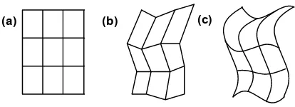
A representation of the topology and geometry A representation of the data defined over the topology Most systems and practitioners use the word geometry to refer to the first component, few use the word topology. It is important to realize that the two concepts are distinct. The study of topology arose from the observation that some problems depend only on “connection” properties (such as adjacency and containment) and not the geometric properties (such as shape or size). For example, Figure 3 shows three geometric realizations of the same topological grid. Topology involves only the properties of neighborhoods of points and not absolute positions in a metric space. Our data model makes the same distinction, and does not require absolute positions in space nor time. This approach reduces the complexity of the data model; geometric data require no special treatment. We view geometric data as just that – data. We claim that grid topology is the distinguishing feature of scientific data, and the only feature requiring specialized solutions. All other data can be modeled as functions over the topological elements.

(a) (b) (c)

Figure 3.Three geometric realizations of one grid.

2.1. Grids

In this section we present the data model over which we will define our language. The fundamental unit of ma-nipulation is the grid. Intuitively, grids are constructed from nodes and connections among the nodes. A sequence of nodes declared to be connected form a cell. A cell is interpreted as an element of some particular dimension. We allow cells of combination of dimensions to be grouped together as a grid. There is a significant flexibility with this construction. We can distinguish between grids made up of just triangles and nodes, versus grids made up of triangles, their edges, and nodes. In fact, grids may be constructed from any combination of nodes, edges, faces, etc. We have chosen simplicity and flexibility at the expense of allowing some odd grids.

Definition A 0-cell or node is a named but otherwise featureless entity.

Definition A k-dimensional cell, denoted k-cell (Berti, 2000) or just cell, is a sequence of 0-cells plus an associated positive integer dimension k. The dimension of the k-cell is constrained, but not defined, by the number of nodes used to represent it. Specifically, if n is the number of nodes in the sequence, then n = 1 implies k = 0, and n > 1 implies k < n. To obtain the nodes that define a k-cell c as a set rather than a sequence, we write V(c).

Intuitively, a 1-cell is a line segment, a 2-cell is a polygon, a 3-cell is a polyhedron, and so on. The number of nodes in a k-cell is not fully specified in order to allow non-simplicial polytopes such as squares and prisms. (A simplex is the polytope of a given dimension requiring the fewest number of nodes. The 2-dimensional simplex is the triangle. The 3-dimensional simplex is the tetrahedron.) To interpret a sequence of nodes as a particular shape, implementations require that a cell type be assigned to each sequence. In this paper, we will assume that cell types are determined and maintained at the physical layer without explicit guidance from the data model.

Definition A gridG is a sequence [G0, G1, …] where Gk is a set of k-cells. A grid must be well formed: There can be no k-cells in Gk that reference a node that is not in G0. The dimension of a grid is the maximum k of all cells in the grid.

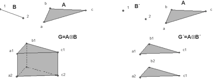
In the diagram at the left of Figure 4, the 2-dimensional grid A has three 0-cells, three 1-cells, and one 2-cell. The 1-dimensional grid B has two 0-cells and one 1-cell. Note that a grid consisting of only nodes is 0-dimensional.

Intuitively, a grid partitions a space into cells of various dimensions. Note that this definition is purely combinatorial; we have not described the space in which the grid is embedded. More precisely, we have not specified a geometric realization for the cells. Geometry in our model is captured as a gridfield, which we will describe in the next section. One final definition gives the relationship between k-cells that share nodes. The notion of incidence captures the intuition that we should be able to retrieve the cells that “touch” a given cell.

Definition A cell c is incident to another cell e, written cpe, if all of the nodes referenced by c are also referenced by e. That is, cpe if V ( c )⊆V ( e ).

Equivalence and containment relationships between two grids can be derived from the definition of incidence. To maintain such a relationship, the implementation must establish a 1-1 correspondence between the nodes of the two grids, and then inspect the induced incidence relationships between the cells of other dimensions. Arbitrary grids will not often be tested for equivalence or containment, however. We have found that many grids can be derived from just a small set of base grids. Keeping track of the relationships between grids amounts to keeping track of the derivations performed on this small base set. Therefore, equivalence and containment can be inferred by a comparison of derivations rather than an expensive cell-by-cell comparison of grids. Reasoning about derivations in this manner is very difficult without a simple data model and simple operations.

Before we describe how to associate data values with a grid to create a gridfield, we introduce operators for manipulating grids themselves.

2.2. Cross Product

The cross product of two grids generates a higher dimen-sional grid based on cross products of their constituent sets of cells.

Consider two zero-dimensional grids, A and B, each containing a single node a and b respectively. Their cross product, A⊗B, would be a new grid also with a single node, which we refer to as ab. If B consisted of two nodes, b1 and b2, then A⊗Bwould consist of two nodes, ab1 and ab2. If B additionally had a 1-cell (b1, b2) then the cross product would have the nodes ab1 and ab2, and one 1-cell connecting them, written (ab1, ab2).

A less trivial example is shown at the left of Figure 4. Intuitively, we are generating a prism from a triangle and a line segment. In our notation, we have

B

_´

A

A

B

1

2

1

2

a b

c

a b

c

a1

b1

c1 _a1

b1

c1

a2 _a2

b2

c1 c2

A

G

G=A

⊗

B

B

_G

_´

G

´

=A

_A

_´

⊗

B

´

_B

_´

{

}

The cross product operation is denoted

G= ⊗A B (2)

Evaluating these expressions, we obtain

0 1 2 3

The 3-cell in the new grid is a prism, resulting from the triangle in A2sweeping out a solid in the third dimension. The 2-cells in the new grid might be triangles or parallelograms, depending on how they were derived. The edges in A1and the edges in B1 together form parallelograms in G2, while the triangles in A2 and the nodes in B0 form triangles in G2.

The product operator introduces a kind of “regularity" (Haber et al., 1991) even if the two component grids are irregular. Consider an extension of the example at the left of Figure 4, in which a 2-dimensional irregular grid in the xy plane is repeated in a third dimension z. The triangles in the xy plane form prisms as they sweep out a space in z. The edges of the triangles will sweep out rectangles. The nodes will sweep out lines. Now we have a true 3-dimensional grid that

is usually classified as “irregular" in visualization applica- tions. But it is important to note that at every z coordinate, the xy grid is the same. We can sometimes exploit this knowledge about how the grid was constructed to map values from one grid to another efficiently.

The cross-product operation is more flexible than might be immediately apparent. The operation at the right of Figure 4 illustrates the cross product of A and a 0-dimensional grid B'. A similar grid arises in the CORIE domain, since the solutions to the governing differential equations are not actually solved in three dimensions. Since the river dynamics are dominated by lateral flow, the equations are solved in two dimensions, but at each depth in the vertical grid. Data values associated with the z dimension cannot be unambiguously assigned to the prisms in the new grid. For a grid of n nodes in the z dimen-sion, there are n triangles, but n – 1 prisms. Our model exposes this potential ambiguity; other models force an assumption about how the data values will be assigned.

2.3. Union and Intersection

The union of two grids can be used to model overlapping or piecemeal grids. For example, in the context of our estuarine simulation, atmospheric condi- tions are inputs

(forcings) to the domain of the solution. The data for these

forcings are a combination of overlapping grid functions provided by two universities’ atmospheric models. Each is defined on a separate grid. The union operation allows reasoning about these two grids as one. The union operator might also be used when partitioning and recombining grids in a parallel environment, or to bring the interior of a grid (say, sets of nodes and triangles) together with a representation of its boundary (a set of edges).

Formally,

The intersection operator is often used to reduce one grid based on the k-cells in another. Frequently, intersection is used only on grids of equal dimension, though the definition does not enforce this limitation. We will use grid intersection to define the merge operator over gridfields in Section 0.

B

to data values.

Definition A gridfield, written Gk g

, is a triple (G, k, g) where g is a function from the k-cells of G to data values. The type of a gridfield, written t[Gk

g

] is the return type of the function g.

The primitive types we will work with in this paper are Integers, Floats, Strings, and Booleans. We will also make use of sets and tuples.

Definition A tuple is a sequence of values of possibly different types. The tupling function tup takes n arguments and generates an n-tuple, unnesting if necessary. For example, tup( , ,a b x y, )= a b x y, , , . (Note that we use angle brackets

to enclose tuples.) In our notation, the singleton tuple x is

identical to the value x.

We adopt the database convention of accessing tuple components by name rather than by position. This named

perspective effectively makes the order of the tuple

compo-nents irrelevant. In the functional programming community, record structures have been proposed that use a similar mechanism. Selector functions (Jones et al., 1999) such as “salinity” or “velocity” are used to access the elements of a record type rather than using positional access functions such as “first” or “second”.

In our domain, gridfields are primarily used to model the physical quantities being simulated. In one version of the CORIE output data, salinity and temperature values are defined over 2-cells at each depth of a product grid like that at the right of Figure 4. Velocity is defined over the nodes (0-cells) in the same grid. Water elevation is a gridfield over the 2-cells of the horizontal two dimensional grid. In a more recent version, the data values are associated with the nodes of the grid rather than the 2-cells. This change had drastic consequences: All the code in the system had to be meticulously checked for dependence on the earlier data format. Our model is able to capture the difference between these two configurations very precisely, exposing affected data products and guiding solutions.

The geometric coordinates that position a node in some space are modeled as data too, constituting their own gridfield. Specifically, a geometric realization of the CORIE grid is given by a gridfield over 0-cells of type

:float, :float, :float

x y z . Geometric data can be associated

with more than just 0-cells, however. Curvilinear grids can be represented by associating a curved interpolation function with each 1-cell. Figure 3 shows three different realizations of the same grid; Figure 3c shows such a curvilinear grid. Many systems do not support this kind of geometric realization; geometric data is associated with the nodes only (as coordinates) and geometry for higher dimensional cells is linearly extrapolated from the cells coordinates. The flexibility and uniformity obtained by modeling all data as functions is a primary strength of this model. Grids of arbitrary dimension, with arbitrary geometry, can be modeled, manipulated, and reasoned about just as easily as simple, low-dimensional grids.

3. Language

In this section we present four operators over gridfields that together can express a variety of data products. In Section 0, we will give examples from the CORIE data product suite to provide illustrations of the language’s expressiveness. First we give a short intuitive description of each operator.

The bind operator associates data to a grid to construct a gridfield.

The merge operator combines multiple gridfields over the intersection of their grids.

The restrict operator changes the structure of a gridfield by evaluating a predicate over its data.

The aggregate operator transforms a gridfield by mapping it onto another grid and aggregating as appro-priate.

We envision other operators being defined as the need arises, but these represent the core language.

3.1. Bind

The bind operator constructs a gridfield from a grid and a function. Implementations of gridfields will not always use a literal function. If our datasets are stored in files, a function implementation might have to open the file, seek to the correct position, read the value, and close the file on each call. For efficiency, we would prefer to read in a large block of values at a time. However, the function abstraction is appropriate for defining our gridfields at this level of abstraction. As long as such a function could be defined, this model is appropriate.

Definition Let A be a grid and f be a function from Ak to data values. Then bind(A, k, f) = Ak

f

where Ak f

is a gridfield. The definition may seem trivial since we simply form a triple from the three arguments. However, this operator has significance in an implementation as a constructor of gridfields. The bind operation can encapsulate a procedure to validate data availability, create indices, or otherwise prepare the values for manipulation as a gridfield. In our model, bind

is just a declaration that the data values represented by the function f match the grid given by G. Note that the same function can be bound to different grids, as long as they share the same set of k-cells.

3.2. Restrict

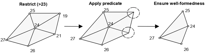
The restrict operator takes a predicate over the data val-ues of a gridfield and filters out k-cells associated with values that do not satisfy it. A frequent use of restrict in our experience is to “zoom" in on a particular region by filtering out those cells whose geometry places them outside a bounding box. Note that since geometry is simply data in our model, this “zoom" operation is treated identically to other filtering operations.

reference removed nodes (Figure 5).

Definition Let Ak f

be a gridfield, where f is a function from Ak to data values of type t. Let p be a predicate over data values of type t. Then restrict(p)[Ak

f

] returns a gridfield Gk

f

. In the case k>0 , G=G G0, 1,...,Gn , where

{ | , ( ) }

k k

G = e e∈A p f eo =true and Gi=Ai for all i≠k.

In this definition, the predicate p is used to filter out some cells of dimension k, but all other cells are included in G. (Note that

o

denotes function composition.) In the case

0

=

k , Gk is defined as before but we must ensure well-formedness by removing any cells that reference deleted nodes. That is, Gi={ |e e∈Ai,∀ ∈v V e p f v( ), o ( )=true} for all i≠k.

3.3. Merge and Cross Product

The merge operator combines two gridfields over the intersection of their grids. More precisely, merge computes the intersection grid of its two arguments, and produces a gridfield over that intersection that returns pairs of values. If the two grids are equal, as they can frequently be in our experience, then merge simply pairs the values from each argument but leaves the base grid unchanged. Figure 6 shows an illustration of this operator.

Definition Let Ak f

and Bk g

be gridfields. Then merge [Ak f

, Bk

g ] = Gk

h

where G=(A∩B), and h e( )= f e g e( ), ( ) for every cell e∈A_i∩B_j.

Merge is related to the intersection operation over the underlying grids. Similarly, we can lift the cross product operator defined for grids and redefine it for gridfields.

Definition The cross product of two gridfields, written Ai

f _⊗ Bj

g

is a gridfield Gk h

where G = A⊗ B, k = i + j, and ( ) ( ), ( )

h e = f e g e for e∈_Ai and c∈B_j.

The union operator can also be applied to gridfields. However, there are some technical complexities, and we omit the formal definition here.

3.4. Aggregate

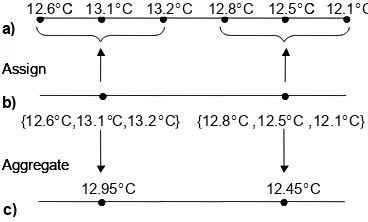
The most expressive operator in our language is aggre-gate. Most significant manipulations involve one or more aggregate operators. As the name implies, aggregate is used to combine multiple values from one gridfield into a single value in another grid. There are two steps to the process. First, a source gridfield's domain is mapped to the target gridfield's domain. An assignment function takes a k-cell from the target grid and returns a set of j-cells in the source grid. Next, all the source cells mapped to a particular target cell are aggregated

Figure 5. Illustration of the merge operator. 27

25

24

26

27

25

24

26

Apply predicate Ensure well-formedness

27

25

24

26

21 19

Restrict (>23)

(x2,y2,z2)

(x4,y4,z4)

(x3,y3,z3) z2

z4

z3 (x2,y2)

(x4,y4) (x1,y1)

(x3,y3)

merge

using an aggregation function.

Consider a timeseries of temperature values for a par-ticular point in the river. We partition the time dimension using a 1-dimensional source grid S, as shown in Figure 7a. One use of the aggregate operator is to perform a “chunking” operation to coarsen the resolution of the grid. The assignment function assigns each node in the target grid T a set of n nodes, the “chunk,” in the source grid S (Figure 7b). The aggregation function then, say, computes the arithmetic mean of the n nodes to obtain single value (Figure 7c).

12.1°C 12.6°C 13.1°C 13.2°C 12.8°C 12.5°C

12.95°C 12.45°C

a)

Assign

Aggregate b)

c)

{12.8°C ,12.5°C ,12.1°C} {12.6°C,13.1°C,13.2°C}

12.1°C 12.6°C 13.1°C 13.2°C 12.8°C 12.5°C

a)

Assign

Aggregate

b)

c)

{12.8°C ,12.5°C ,12.1°C} {12.6°C,13.1°C,13.2°C}

Figure 7. Illustration of the aggregate operator.

Definition Let T be a grid and Sj g

be a gridfield of type a. Let f be a function from sets of values of type a to values of type b. That is, f :

{ }

a →b. Let m be a function from Tk to sets of cells in Fj. That is, m T: k→

{ }

Sj . Then aggregate (T,

k, m, f)[Sj g

] produces a gridfield Tk h

where h= f o og m. By abuse of notation, the function g is applied to each member of the set returned by the function m. We call T the target grid, S the source grid, m the assignment function, and f the aggrega-tion funcaggrega-tion.

Note that the aggregate operator accepts two user-defined functions as arguments. This design makes the operator very flexible, but also burdens the user with function definition. The assignment function in particular seems that it might require significant ingenuity to define. However, the algebraic properties of our language admit some relief. Since our language allows reasoning about how grids are constructed, relationships between the cells of two different grids can often be defined topologically and simply.

For example, consider the CORIE grid described in Sec-tion Error! Reference source not found.. We crossed an unstructured 2-dimensional grid (the horizontal grid) in the xy plane with a 0-dimensional grid consisting of points along the z axis (the vertical grid). We noted in Section 0 that this grid should not be considered fully unstructured, though it would be considered so in most visualization applications. Instead, we want to exploit the fact that the xy grid is duplicated for every node in the z grid.

If this grid were modeled as fully “irregular,” the rela-tionship between the cross product grid and the horizontal grid is lost. Imagine we want to project the values in the cross

product grid down onto a horizontal “slice” to compute the maximum value in each vertical column. To assign the nodes of the cross product grid onto the nodes in the horizontal grid, most systems appeal to the geometry data. Specifically, for each node in the horizontal grid, existing tools must scan every node in the full cross-product grid to find those cells with matching xy coordinates. With our operators, we can derive the fact that the horizontal grid is related to the full grid via the cross product operator. We can use this relationship to define the assignment function as the cell product, avoiding a scan of every node in the full grid. Our experience working on the CORIE project has shown that many of the grids found in practice are topologically related to just a few “base” grids. Since grids are first-class in our language, we are better able to model and exploit these topological relationships to simplify and accelerate our recipes.

Not every pair of grids exhibits a simple topological re-lationship, however. Sometimes it is necessary to scan the source or target grids and relate cells using data values. As we mentioned in the last paragraph, such data-oriented as-signment functions can involve extensive iteration; no shortcuts based on topology are applicable. In these cases, our model does not perform better than existing tools. However, pinpointing the cause of the inefficiency as the assignment task helps guide further analysis. In existing software, the assignment step and aggregation step cannot be reasoned about separately, obscuring the cause of inefficiencies.

Figure 8. Illustration of the CORIE vertical grid.

To further alleviate the burden of defining assignment functions (purely topological or otherwise), we offer several special cases of the aggregate operator, and promote them as operators themselves. Each of the following can be defined in terms of the aggregate operator.

The apply operator assigns each k-cell to itself and then applies a function to the k-cell’s data value. Intuitively, apply simply applies a function to each value of the grid, and forms a new gridfield with the results.

The affix operator changes the domain of the gridfield from j-cells to k-cells, applying a function to aggregate the results. This operator can transform node-centered datasets into cell-centered datasets.

The project operator is similar to the project operator in the relational algebra. One provides the names of the data values of interest given by a tuple-valued gridfield, such as “velocity” or “salinity,” and all remaining data values are removed.

4. Examples

In this section we describe and analyze two data products used in the CORIE system. We will show how they can be expressed as gridfield manipulations and optimized using rewrite rules.

First we must construct the full grid over which the CORIE simulations are computed. Figure 1 shows the 2-dimensional component of the full CORIE grid. Figure 8 shows the 1-dimensional component. Our plan is to compute the cross product of these two component grids. Note, though, that the vertical component in Figure 8 could also be represented as a 0-dimensional grid; just a set of nodes. We gave an example in Figure 4 of the effect this change has on the result of the cross product operator. Using the 1-dimensional vertical grid, we obtain a 3-dimensional grid constructed from prisms, faces, edges, and nodes. Using the 0-dimensional version of the vertical component, we obtain a “stacked” grid, with the 2-dimensional component repeated at each depth. Both of these product grids are used at various times during the CORIE simulation. Our model admits expression of both grids precisely and uniformly.

For the purposes of this example, we will assume the vertical component is 0-dimensional. Indeed, let H be the horizontal CORIE grid and let V be the vertical CORIE grid. Then

,

0 2

[ , , , ...]

H= H H∅ ∅

0

[ , , ...]

V = V ∅ (7)

The full CORIE grid is then

G=H⊗V

0 0 2 0

[ , , , , ...]

G= H ×V ∅ H ×V ∅ (8)

Although the simulation code operates over this grid, the solution is produced on a smaller grid. To see why, consider Figure 8 again. The shaded region represents the bathymetry of the river bottom. The horizontal grid is defined to cover the entire surface of the water. At depths other than the surface, some nodes are positioned underground! The simulation code takes this situation into account and produces only valid, “wet,” data values to conserve disk space. We must define this “wet" grid to obtain an adequate description of the topology of the data. The bathymetry data is represented as a river bottom depth (a float) for each node in the horizontal grid. Therefore, we model bathymetry as a gridfield over the horizontal grid H. To filter out those nodes that are deeper

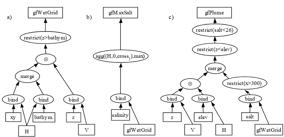
than the river bottom, we need to compare the depth at a node in the product grid G with the bottom depth at the corresponding node in H. Figure 9 shows this construction using grid operators.

We point out a couple of details about Figure 9. The predicate in the restrict operator is expressed in terms of selector functions. Given a 0-cell e, the function component of gfFullGrid will return a value xy

( )

e ,bathym

( ) ( )

e ,z e . Passing this function compo- nent to the selector function z

returns the third element in the tuple, z(e).

The gridfield gfWetGrid returns 3-dimensional coordi-nates and bathymetry information for each 0-cell in the grid. The only nodes in the grid are those above the bathymetry depth of the river at each point. The grid component of gfWetGrid is now ready to be bound to data values supplied by the simulation.

Maximum Salinity. The first data product we will ex-press using this grid is a 2-dimensional isoline image of the salinity in the Columbia River Estuary. An isoline image draws curves representing constant values in a scalar field. In CORIE, 3-dimensional gridfields for salinity and temperature are projected down to two dimensions by aggregating over depth and computing the maximum and minimum. Figure 2a shows an example of this data product. Figure 9b gives the recipe for the maximum salinity over depth.

The function crossj returns all the cells in one vertical column of the 3-dimensional grid. An aggregation operation that uses crossj as an assignment function produces a gridfield over the 2-dimensional horizontal grid. The value associated with each node is the maximum salinity found in the vertical column of water located at that node. Figure 2a could be generated by applying a contouring algorithm directly to this data. In fact, even this contouring operation can be modeled as an aggregation with a simple assignment function and an aggregation function that associates a line segment with each 2-cell.

Plume Volume. The second data product we will de-scribe is a calculation of plume volume. The plume is defined as a region of water outside the estuary that exhibits salinity below a given threshold. This definition implies that to obtain the plume portion of the grid, we must cut away the river portion, and then cut away the portion of the grid with salinity values above the threshold.

Before these cuts, though, we must cut away the portion of the grid that is above the surface of the water just as we did for the underground values. We have simplified the discussion by considering only a single point in time. In practice, we would use another cross product to incorporate the 1-dimensional time grid, since the surface elevation changes over time, unlike most models of river bathymetry.

bind the salinity function to the grid computed in Figure 9a, and apply a predicate on x to extract the ocean portion of the grid. Next, we merge the two gridfields and apply the two remaining predicates to filter out those cells positioned above the water's surface and those with a salinity value 26 psu or greater.

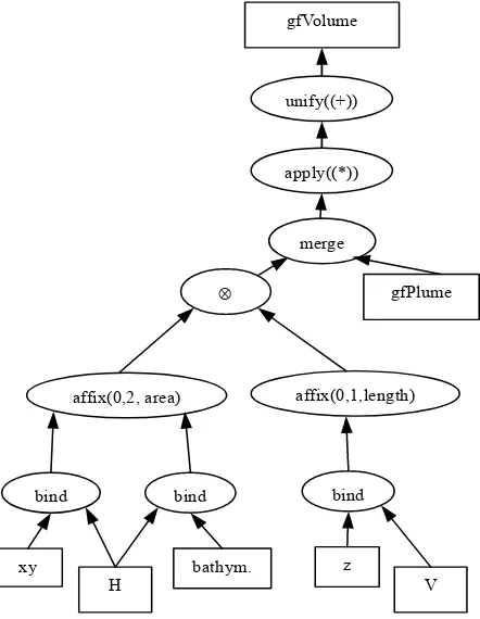
The gridfield gfPlume returns a 6-tuple x, y,z,bathym,elev,salt defined over the nodes. To compute the volume, we must calculate the volume of each prism in the grid, and sum the values. We have some choices of how we might do this. One way would be to 1) use project to remove everything but the (x,y,z) coordinates, and 2) use affix

to produce a gridfield over prisms that returned 6-tuples of (x,y,z) coordinate triples representing the corners of the prism, and 3) use apply along with a specialized function for computing the volume of prisms. However, let us assume that we do not have such a function available. We can still compute the volume using the fact that our grid is a cross product of two simpler grids and not just an unstructured assemblage of prisms. (Along with the assumption that the (x,y,z) values refer to a Cartesian coordinate frame.)

Figure 10 illustrates the technique. We use affix to move the data values from the nodes to the 2-cells and 1-cells on the horizontal and vertical grids respectively. We allow the affix operator to apply an aggregation function to the values after they are assigned. In this case, we compute the area of the triangles and the length of the line segments.

Next, we compute the cross product of these gridfields, producing a gridfield that returns pairs, area,length for

each prism. (Refer to the definition of the cross product of gridfield.) We then merge the new gridfield with gfPlume to remove the prisms not in the plume. Finally, we can multiply

length by area using the apply operator to compute the volume of each 3-cell, then sum those up with the unify

operator.

With these examples, we hope to demonstrate the flexi-bility and simplicity of designing data products using our framework. There was no discussion of how to iterate over particular data structures, but we were precise enough to specify the data product completely. Note also how we re-used recipes: gfPlume appears in both Figure 9 and Figure 10. Since the same data products are often generated for each run of the simulation, we envision the entire data product suite being expressed and browsed as one large network of operators. Such a network admits global reasoning, something very difficult when the data products are simply unrelated scripts and programs.

Another aspect of these examples we wish to point out is our use of operator tree diagrams. These diagrams are common in database query processing literature, and are very helpful when reasoning about complex manipulations.

5. Analysis

One’s ability to reason about expressions in a language is a function of the number of operators available and complexity of the operators themselves. Reasoning about VTK and DX programs is complicated by the hundreds of different operations and their interdependent semantics. We bind

H bind

mer ge

bind

V

⊗

xy bathy m. z

restrict(z>bathy m) gfW etGrid

gfW etGrid bind

agg((H,0,cross_j),max)

gfM axSalt

salinity

gfW etGrid salt

restrict(x>300)

H bind

elev mer ge

⊗

V bind

z

restrict(z<elev) restrict(salt<26)

bind gfPlum e

a) b) c)

Figure 9. Recipes to compute (a) the valid (“wet”) portion of the CORIE grid, (b) the maximum salinity over

have attempted to provide a language that more naturally supports reasoning about correctness and efficiency. We use four fundamental operators to express a wide range of data products. We can also model details of the grids that other approaches do not capture, such as arbitrary dimension, shared topology, and implicit containment relationships. Our operators also have reasonably intuitive semantics, though the complexity of the problem space does infect some definitions. Together, these language properties allow us to perform some reasoning tasks that are difficult with large, cumbersome libraries of highly-specialized algorithms. To illustrate the kind of reasoning tasks supported by the language, we consider the execution and optimization of a portion of the plume recipe in Figure 9.

Figure 10. Computing the plume volume using the cross product operator.

bind

H bind

affix(0,2, area)

bind

V ⊗

xy bathym. z

gfVolume

gfPlume merge

apply((*)) unify((+))

affix(0,1,length)

Consider Figure 11, a diagram based on a portion of the plume computation in the last section. The boxes represent gridfields over the full CORIE grid with salinity and geometry information. The ovals are operators; m is a merge operator, and r is a restrict operator (with r(X) denoting a predicate over the grid X). Figure 11b is a recipe fragment directly taken from Figure 9c. The other figures are equivalent recipes generated by applying an algebraic identity, namely that

merge and restrict commute.

Readers versed in relational query processing might be tempted to guess that Figure 11b is the best choice for

evaluation. The restrict operator appears similar to a rela-tional select, and the merge operator appears similar to a relational join. A common relational database optimization technique is to “push selects through joins,” to reduce the size of the inputs to the join. However, consider the fact that we know that the two base gridfields are defined over the same grid. If the grids S and X in Figure 11are equivalent, then the

merge operator does not need to do any work to compute their intersection. Treating the merge operator as a join is not appropriate in this case. If we place the restrict operators after the merge operator and combine them (Figure 11a), we might avoid an extra traversal of the grid S = X.

m a)

Ss _Xx

r(s,x) m

r(s) b)

Ss _Xx

r(x)

m c)

Ss _Xx

r(x) r(s)

Figure 11. Three equivalent recipes.

Now we will look more closely at how we might evaluate the restrict operators. One option is to bring the entire dataset into memory, compute the restriction, and then pass the reduced grid and its data on to the next operator. Another option is to bring the grid into memory one cell at a time, retrieve the data value associated with that cell, and evaluate the predicate on the data value. If the value satisfies the predicate, then its cell and value are passed on to the next operator. We refer to the latter technique as pipelining, and note that it is a common technique in database query evaluation.

Since we are computing plume volume, we no longer need the geometry data once we have restricted the grid to the ocean portion. After this operator, we can remove the geometry data from memory, admitting a possible perform-ance boost. In our language, we would accomplish this task using a project operator. If we do project out the unneeded data, we avoid handling both the salinity data and the geometry data in memory at the same time. We also do not sacrifice the simple, constant-time evaluation of merge. Although the grids are not equal, the ocean grid is guaranteed to be a subgrid of the full salinity grid. The merge operator can just replace the full grid with the reduced grid, which amounts to reducing the domain of the salinity function. So, it is plausible that Figure 11c is the best choice.

would be difficult.

A prerequisite to the kind of analysis we applied in this example is the ability to trace the propagation of data properties through an expression. This task amounts to tracing the property inductively through each operator. Table 1 shows two properties, grid and size, of the output of each operator in the language.

Estimating the size of intermediate results is helpful when considering which of several equivalent recipes will re-quire the least amount of work. We estimate the size of a gridfield as the number of domain elements its grid contains, multiplied by the arity of the tuple in the function's type. If a gridfield returns a tuple of three values, such as x,y,z , the arity of the tuple is simply three. In general, the arity of a tuple type is just the number of elements in the sequence. The arity of other primitive types is one. This estimate of size is somewhat simplistic, but it does provide an indication of which operators in a recipe will do the most work.

6. Related Work

Related work is found in the visualization community, database community, and in the projects developing special-ized scientific data management systems.

Data Models. Many scientific data models, especially for visualization, have been proposed over the last decade and a half. Butler and Pendley applied fiber bundle structures found in mathematics and physics to the representation of scientific data to support visualization (Butler et al., 1989; Butler et al., 1991; Haber et al., 1991; Treinish, 1999). Fiber bundles are very general topological structures capable of modeling many diverse classes of objects such as simple functions, vector fields, geometric shapes such as tori, and visualization operations.

Fiber bundles showed great promise in their generality and support for formal reasoning. However, limitations to their direct use for scientific data modeling appeared. First, fiber bundles were developed to model continuous fields (manifolds), and do not address the discrete nature of

computational grids (Moran, 2001). Second, much of the expressive power of fiber bundles is derived from complexities that most scientific grids do not exhibit. Most scientific grids are cast as “trivial” fiber bundles – simple Cartesian cross products – that do not make use of the full fiber bundle machinery.

Scientific Data Management Systems. Scientific data manipulation has also been studied in the context of data management. Some systems do not attempt to model the contents of datasets, but just provide support for querying the files and programs that produce them (Frew and Bose, 2001; Foster et al., 2002; Wolniewicz, 1993). Metadata attached to programs allows tracking of data provenance – the information about how the data was produced. Users of the Chimera system (Foster et al., 2002) can register their programs and inputs and allow Chimera to manage execution. This facility gives rise to a notion of virtual data that can be queried before it has been derived.

Our work differs in two ways. First, these systems model datasets and manipulations coarsely as indivisible files and codes; we model the contents of the datasets and the patterns of manipulations over them. Systems that rely on user-defined programs are vulnerable to data dependence problems and do not help ease the programming burden. Second, our work in this paper does not tackle scientific data management as a whole, though our project includes data management in its scope and vision.

Scientific Visualization Systems. There also have been efforts to develop combined scientific data management and visualization systems. The Active Data Repository (ADR) (Kurc et al., 2001) optimizes storage and retrieval of very large multidimensional datasets, including gridded datasets. Queries over the data involve three transformations related to our operators: selecting a subregion, mapping one grid onto another, and processing the results. ADR is highly customized for particular domains. New C++ classes are developed for each application.

Our work aims to formalize intuitions about grid map-pings, grid selections, as well as several other operations frequently encountered in scientific applications. We also advocate a declarative approach that identifies the commonalities across scientific data applications, rather than

Table 1. Output properties of core operators

Operator Expression Output Grid Output Size

bind bind(G,k,f) G |G_k |arity f( )

merge merge[Aif, Bjg] A∩B |A_k ∩B_k |(arity(f))

cross product A_if ⊗B_jg A⊗B | Ai ||Bj |(arity(f)+arity(g))

restrict restrict(p)[ Akg] depends on predicate less than | Ak |

specializing low-level code on a per-application basis.

Arrays Types for Databases. The database community has investigated query language extensions supporting fast collection types, often citing scientific data processing as a motivation (Marathe and Salem, 1997; Libkin et al., 1996; Fegaras and Maier, 1995). However, the ubiquity of arrays in the scientific domain is not necessarily evidence that arrays constitute an appropriate data model for scientific analysis, but rather that more specialized data models have not been developed. Further, direct use of arrays and other low-level data structures lead to data dependence problems. Declarative data languages have provided a solution to data dependence by avoiding such structures. Rather than make one’s data language more procedural, we recommend making one’s application language more declarative.

Geographic Information Systems. Superficially, geo-graphic information systems (GIS) (Eastman, 1997; Dewitt et al., 1994) research seems closely related to our work. Applications in both areas involve representations of data objects physically positioned in some space of values. Applications in both areas frequently make use of range queries, where intervals in space are used to locate relevant objects.

However, GIS are designed for a particular class of data objects that does not include gridded datasets. Spatial databases model and manage data objects that have a spatial extent, while our work is to model spatial extents over which data has been defined. In our domain, gridded datasets are manipulated as a whole; finding objects located in space is a secondary concern.

Raster GIS (Câmara, 2000; Widmann and Bauman, 1997; Eastman, 1997) do manipulate grid structures, but they use primarily structured grids. Grids are not considered first-class and are difficult to reason about independently of the data.

Data models based on simplicial complexes, have been proposed for GIS (Jackson, Egenhofer, and Frank, 1989) to model a domain related to ours – datasets embodying solutions to numerical partial differential equations (Berti, 2000). Simplicial complexes provide a formal topological definition of grids. Our model allows cells to be other polytopes besides simplices, but also sacrifices the mature theory of simplicial complexes.

7. Conclusions and Future Work

Our motivation for formalizing grid manipulations is de-rived from our more general interest in scientific data management. We have observed that there are two funda-mental tasks in scientific data processing: one to retrieve datasets of interest and one to analyze those datasets, pro-ducing data products. The first task requires that datasets be identified using metadata such as dates, times, user names, simulation parameters, and annotations. These kinds of data are relatively well understood and are naturally modeled using relational or object-relational systems. Datasets can then be retrieved using the available query languages. The second task, however, generally requires the use of highly specialized

applications or customized code. Our eventual goal is to integrate the two tasks into one declarative language. In this paper, we described our research into a language for the second task. Our conclusion is that such a language can be defined, and that only five core operators are necessary to express all of the existing CORIE data products.

We have also used operator expressions as a common framework for comparing the capabilities of different software systems. For example, we can describe precisely the difference between how VTK and DX implement a restrict

operation. VTK provides a “Threshold” object that behaves much as we have described restrict. DX, however, recommends marking restricted cells as “invalid” and then filtering them out only in the final rendering. DX’s construct is therefore a straightforward use of the aggregate operator. The differences between such routines become clear when cast as expressions in our language.

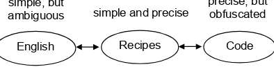
The language has also shown promise as an intermediate specification language between English descriptions of data products and programming language implementations. Data products are usually first expressed in English for ease of discussion. However, these descriptions are much generally much too ambiguous to use to generate an executable program. Correct implementations are necessarily precise, but the simple conceptual description of the data product is lost in obtuse code. Our “recipes” are simple enough to maintain clarity, but precise enough to reason about correctness, efficiency, and their relationship to the rest of the data product suite. Figure 12 illustrates this idea.

English Recipes Code

simple, but

ambiguous simple and precise

precise, but obfuscated

Figure 12. Means of describing data products.

Finally, we list several specific features of our language that distinguish it from existing tools.

Grids are first-class structures (see Section 1), allowing grids to be shared between datasets and manipulated independently.

Grid geometry is modeled as data, simplifying the model and allowing grids to be manipulated using purely topological operators such as union, intersection, and cross product.

The cross product operator is used to express complex grids simply and precisely.

Grids of arbitrary dimension can be defined and ma-nipulated.

Functions abstractions allow independence from choosing a particular data representation.

Although specialized processing is necessary for most scientific applications, our operators clearly separate custom code from core operator functionality. Specifically, assignment and aggregation functions capture all customiza-tions we have required thus far, save for the predicates passed to restrict.

Equivalent recipes can be generated using algebraic identities and compared by analyzing the types, grids, and sizes of intermediate gridfields.

There are limitations to the language. Recursive ma-nipulations such as a streamline calculation over vector fields cannot be expressed easily. We are investigating a fixpoint operator to express such manipulations. Also, we have not yet integrated dataset manipulations with more traditional metadata queries.

The language has proved useful for reasoning about the computations in the CORIE system. Our ongoing work is to provide an implementation of the language. The planned implementation will involve two technologies: a functional programming language for working with the abstract operators, and a fast low-level language for the physical operators. VTK is an appropriate starting point for the physical layer; the algorithms are state of the art, and the library is robust and well maintained. However, as discussed in Section 1, the library will need to be extended with several custom operations. For the logical layer, we plan to use the functional language Haskell (Peyton-Jones et al., 1999) to manipulate abstract grids and gridfields.

References

Baptista, A.M., McNamee, D., Pu, C., Steere, D.C. and Walpole, J. (2000). Research challenges in environmental observation and forecasting systems, in Proc. of the 6th Annual International Conference on Mobile Computing and Networking, Boston, MA, USA.

Berti, G. (2000). Generic Software Components for Scientific Computing, Ph.D. Dissertation, Faculty of mathematics, com-puter science and natural science, BTU Cottbus, Germany. Butler, D.M. and Bryson, S. (1991). Vector-bundle classes form

powerful tool for scientific visualization. Comput. Phys., 6(6), 576-584.

Butler, D.M. and Pendley, M.H. (1989). A visualization model based on the mathematics of fiber bundles. Comput. Phys., 3(5), 45-51.

Câmara, G., et al. (2000). TerraLib: Technology in support of GIS innovation, in Workshop Brasileiro de Geoinformática, GeoInfo2000, São Paulo, Brazil.

Codd, E.F. (1970). A relational model of data for large shared data banks. Commun. ACM, 13(6), 377-387.

Codd, E.F. (1990). The Relational Model for Database Management: Version 2, Addison-Wesley, MA, USA.

DeWitt, D.J., Kabra, N., Luo, J., Patel, J.M. and Yu, J. (1994).

Client-Server Paradise, in Proc. of the 20th International Con-ference on Very Large Databases, Santiago, Chile, pp. 558-569. Eastman, J.R. (1997). IDRISI User’s Guide, Clark University,

Worchester, MA, USA.

Fegaras, L. and Maier, D. (1995). Towards an effective calculus for object query languages, in Proc. ACM SIGMOD, San Jose, CA, USA, pp. 47-58.

Foster, I., Voeckler, J., Wilde, M. and Zhao, Y. (2002). Chimera: A virtual data system for representing, querying, and automating data derivation, in the 14th Conference on Scientific and Statistical Database Management, Edinburgh, Scotland, UK. Frew, J. and Bose, R. (2001). An Overview of the Earth System

Science Workbench, Technical report, Donald Bren School of Environmental Science and Management University of Cali-fornia, Santa Barbara, CA, USA.

Haber, R., Lucas, B. and Collins, N. (1991). A data model for scientific visualization with provision for regular and irregular grids, in Proc. of IEEE Visualization.

Jackson, J., Egenhofer, M. and Frank, A. (1989). A topological data model for spatial databases, in Proc. ACM SIGMOD, Springer Lecture Notes in Computer Science, Springer Verlag, 409, pp. 271-285.

Jones, M. and Peyton Jones, S. (1999). Lightweight extensible records for Haskell, in Haskell Workshop Proc., Paris, France. Kurc, T., Atalyurek, U., Chang, C., Sussman, A. and Salz, J. (2001).

Exploration and Visualization of Very Large Datasets with the Active Data Repository, Technical report, CS-TR4208, University of Maryland, College Park, MD,USA.

Libkin, L., Machlin, R. and Wong, L. (1996). A query language for multidimensional arrays: design, implementation, and opti-mization techniques, in Proc. ACM SIGMOD, Montreal, Canada, pp. 228-239.

Marathe, A.P. and Salem, K. (1997). A language for manipulating ar-rays, VLDB J., 46-55.

Moran, P. (2001). Field Model: An Object-Oriented Data Model for Fields, Technical report, NASA Ames Research Center, Moffett Field, CA, USA.

OpenDX Programmer’s Reference (2002).

http://opendx.npaci.edu/docs/html/proguide.htm.

Peyton-Jones, S.L. and Hughes, J. (Eds.) (1999). Haskell 98: A Non-strict, purely functional language.

http://www.haskell.org/onlinereport.

Schroeder, W.J., Martin, K.M. and Lorensen. W.E. (1996). The design and implementation of an object-oriented toolkit for 3D graphics and visualization, in Proc. of IEEE Visualization. Treinish, L. (1999). A function-based data model for visualization, in

Proc. of IEEE Visualization.

Widmann, N. and Baumann, P. (1997). Towards comprehensive database support for geoscientific raster data. ACM-GIS, 54-57. Wilkin, M., Pearson, P., Turner, P., McCandlish, C., Baptista, A.M.

and Barrett, P. (1999). Coastal and estuarine forecast systems: A multi-purpose infrastructure for the columbia river. Earth Syst. Monit., 9(3), National Oceanic and Atmospheric Administration, Washington, DC, USA.