APPLICATIONS OF FLUID DYNAMICS BASED
ON GAUGE FIELD THEORY APPROACH
A thesis submitted to the Fakultas Pasca-Sarjana Universitas Indonesia in partial fulfillment of the requirements for the degree of Master of Science
Graduate Program in Pure and Applied Physics
KETUT EKO ARI SAPUTRO 6302020149
Universitas Indonesia
Lembar Persetujuan
Judul tesis : Applications Of Fluid Dynamics Based On Gauge Field Theory Approach
Nama : Ketut Eko Ari Saputro
NPM : 6302020149
tesis ini telah diperiksa dan disetujui
Depok, 29 Juni 2005
Mengesahkan
Pembimbing I Pembimbing II
(Dr. Terry Mart) (Dr. L.T. Handoko)
Penguji I Penguji II Penguji III
(Dr. Agus Salam) (Dr. Imam) (Dr. Anto Sulaksono)
Ketua Program Magister Fisika
Program Pasca Sarjana FMIPA UI
Acknowledgements
I began working on my thesis soon as I joined the nonlinear physics group at University
of Indonesia on July 2004 under supervision of Dr. L.T. Handoko. He was actually
one of the reviewers for my BSc theses at Bogor Institute of Agricultural about the
phenomenon on nonlinear optics. After that, I spent my time to study gauge field
theory (it’s something new for me).
First of all, I would like to acknowledge my primary advisor, Dr. L.T. Handoko for
all guidance, patience and critical comments. I am also indebted to Dr Terry Mart, he
taught me about the quantum mechanics. I thank D r.Anto Sulaksono and Dr. Agus Salam for his intriguing question during my defense. I would like to appreciate our
theoretical group, Albert Sulaiman, Fahd, Jani, Ardi Mustafa, Anton, Freddy, etc for
so many valuable discussion.
The last but not the least, Tri Apriyani, Dhifa al-hakim and Jauza Nur Azizah for
their patience and I always love you all.
My study was supported by Nurul Fikri learning center.
Jakarta, 2005
Abstract
Recently, a new approach to deal with the Navier-Stokes equation has been
devel-oped. The equation which governs the fluid dynamics is a a non-linear one and then
generally unsolvable. In the new approach, the fluid dynamics is described using the
relativistic gauge invariant bosonic lagrangian which could reproduce the Navier-Stokes
equation as its equation of motion through the Euler-Lagrange principle. Based on the
lagrangian we model the fluid dynamics phenomenon as scattering of either three or
four fluid bunches represented by the gauge field Aµ= (φ, ~A)≡ 2d|~v|2 −V,−d~v
with
~v is velocity andd is a parameter to adjust the dimension for any potentialV. Further we present all relevant Fynman rules and diagrams, and also provide complete
calcu-lations for all vertices induced by three and four fluid fields interactions.
Contents
Acknowledgements iii
Abstract iv
Contents v
1 Introduction 1
1.1 Background . . . 1
1.2 Overview . . . 2
2 Navier-Stokes Equation From Gauge field theory 3 2.1 Introduction . . . 3
2.2 Gauge invariant bosonic lagrangian . . . 4
2.2.1 Abelian gauge theory . . . 5
2.2.2 Non-abelian gauge theory . . . 6
2.3 The NS equation from the gauge field theory . . . 7
3 Multi Fluid System Using Gauge Field Theory Approach 10 3.1 Feyman Diagram for Fluid System . . . 10
3.2 Multi Fluids System . . . 12
3.2.1 Interaction of Three Fluids System Dynamics . . . 12
3.2.2 Interaction of Four Fluids System Dynamics . . . 15
B Three points amplitude calculation 24
C Four points amplitude calculation 33
Chapter 1
Introduction
1.1
Background
The understanding of fluid dynamics like hydrodynamic turbulence is an important
problem for nature science, from both, theoretical and experimental point of view,
and has been investigated intensively over the last century. However a deep and fully comprehension of the problem remains obscure. Over the last years, the investigation
of turbulent hydrodynamics has experienced a revival since turbulence has became a
very fruitful research field for theorists who study the analogies between turbulence and
field theory, critical phenomena and condensed matter physics , renewing the optimism
to solve the turbulence problem. The dynamics of turbulent viscous fluid is expressed
by the Navier-Stokes (NS) equations of motion, which in a vectorial form is a fluid flow
described by,
∂~v
∂t + (~v·∇~)~v=−
1
ρ∇~P −ν ~∇
2
~v , (1.1)
where~v is the velocity field, P is pressure, ρ is density and ν is the kinematic viscos-ity. The equation of continuity reduces to the requirement that the velocity field is
divergenceless for incompressible fluids,
~
∇ ·~v = 0. (1.2)
In this context,
univer-integral length-scale of the largest eddies andU is a characteristic large-scale velocity), measures the competition between convective and diffusive processes in an
incompress-ible fluid described by the NS equations. In view of this, the incompressincompress-ible fluid flow
assumes high Reynolds numbers when the velocity increases and, consequently, the
solution for Eq. (1.1) becomes unstable and the fluid switches to a new regime of
a very complex motion with the velocity varying almost randomly and without any
noticeable order. To discover the laws describing what exactly is going on with the fluid in this turbulent regime is very important to both theoretical and applied science.
Recently, A. Sulaiman and L.T. Handoko proposed an alternative approach to treat
fluid dynamics [1]. In the fluid dynamics which is governed by the NS equation we are
mostly interested only in how the forces are mediated, and not in the transition of an
initial state to another final state as concerned in particle physics. Based on lagrangian
density Navier-stokes gauge field theory, they describes the dynamical of interactions
multi fluids system like on particle physics.
LNS=−
1 4F
a µνF
aµν
−gJaµAaµ . (1.3)
In this thesis , we make a further investigation of the physical contents present in that
theory, in order to furnish a better understanding of fluid dynamics.
1.2
Overview
This theses is organized as follow. The introduction and background of the problem
are given in chapter one. Then the theoretical basic of this thesis,i.e.constructing the Navier-stokes equation from gauge field theory, will be described in chapter two. The
Chapter 2
Navier-Stokes Equation From
Gauge field theory
In this chapter we will construct the Navier-Stokes equation from first principle using
relativistic bosonic lagrangian which is invariant under local gauge transformations. We
show that by defining the bosonic field to represent the dynamic of fluid in a particular
form, a general Navier-Stokes equation with conservative forces can be reproduced
exactly. It also induces two new forces, one is relevant for rotational fluid, and the other is due to the fluid’s current or density. This approach provides an underlying
theory to apply the tools in field theory to the problems in fluid dynamics.
2.1
Introduction
The Navier-Stokes (NS) equation represents a non-linier system with flow’s velocity
~v ≡ ~v(xµ), where xµ is a 4-dimensional space consists of time and spatial spaces,
xµ ≡ (x0, xi) = (t, ~r) = (t, x, y, z). Note that throughout the paper we use natural
unit, i.e. the light velocity c = 1 such that ct = t and then time and spatial spaces have a same dimension. Also we use the relativistic (Minkowski) space, with the
metricgµν = (1,−~1) = (1,−1,−1,−1) that leads tox2 =xµxµ =xµgµνxν =x20−x2 =
x2
0−x21 −x22 −x23.
Since the NS equation is derived from the second Newton’s law, in principle it
not clear and intuitively understandable claim since both equations represent different
systems. Moreover, some authors have also formulated the fluid dynamics in lagrangian
with gauge symmetries [4]. However, in those previous works the lagrangian has been
constructed from continuity equation.
Inspired by those pioneering works, we have tried to construct the NS equation
from first principle of analytical mechanics,i.e. starting from lagrangian density. Also concerning that the NS equation is a system with 4-dimensional space as mentioned above, it is natural to borrow the methods in the relativistic field theory which treats
time and space equally. Then we start with developing a lagrangian for bosonic field
and put a contraint such that it is gauge invariant. Taking the bosonic field to have
a particular form representing the dynamics of fluid, we derive the equation of motion
which reproduces the NS equation.
2.2
Gauge invariant bosonic lagrangian
In the relativistic field theory, the lagrangian (density) for a bosonic fieldA is written as [6],
LA= (∂µA)(∂µA) +m2AA
2 , (2.1)
wheremA is a coupling constant with mass dimension, and ∂µ ≡∂/∂xµ. The bosonic
field has the dimension of [A] = 1 in the unit of mass dimension [m] = 1 ([xµ] =−1).
The bosonic particles are, in particle physics, interpreted as the particles which are responsible to mediate the forces between interacting fermions,ψ’s. Then, one has to
first start from the fermionic lagrangian,
Lψ =iψγµ(∂µψ)−mψψψ , (2.2)
whereψ and ψ are the fermion and anti-fermion fields with the dimension [ψ] = [ψ] = 3/2 (then [mψ] = 1 as above), while γµ is the Dirac gamma matrices. In order to
expand the theory and incorporate some particular interactions, one should impose
2.2.1
Abelian gauge theory
For simplicity, one might introduce the simplest symmetry calledU(1) (abelian) gauge symmetry. TheU(1) local transformation1is just a phase transformationU
≡exp [−iθ(x)] of the fermions, that is ψ −→U ψ′ ≡ U ψ. If one requires that the lagrangian in Eq.
(2.2) is invariant under this local transformation,i.e. L → L′ =L, a new term coming
from replacing the partial derivative with the covariant one ∂µ → Dµ ≡ ∂µ+ieAµ,
should be added as,
L =Lψ−e(ψγµψ)Aµ. (2.3)
Here the additional field Aµ should be a vector boson since [Aµ] = 1 as shown in Eq.
(2.1). This field is known as gauge boson and should be transformed under U(1) as,
Aµ U
−→A′
µ≡Aµ+
1
e(∂µθ), (2.4)
to keep the invariance of Eq. (2.3). Here e is a dimensionless coupling constant interpreted as electric charge later on.
The existence of a particle requires that there must be a kinetic term of that particle
in the lagrangian. In the case of newly introduced Aµ above, it is fulfilled by adding
the kinetic term using the standard boson lagrangian in Eq. (2.1). However, it is easy
to verify that the kinetic term (i.e. the first term) in Eq. (2.1) is not invariant under the transformation of Eq. (2.4). Then one must modify the kinetic term to keep the gauge invariance. This can be done by writing down the kinetic term in the form of
anti-symmetric strength tensor Fµν [5],
LA=−
1 4FµνF
µν , (2.5)
with Fµν ≡∂µAν −∂νAµ, and the factor of 1/4 is just a normalization factor.
On the other hand, the mass term (the second term) in Eq. (2.1) is automatically
discarded in this theory since the quadratic term of Aµ is not invariant (and then not
Finally, imposing theU(1) gauge symmetry, one ends up with the relativistic version of electromagnetic theory, known as the quantum electrodynamics (QED),
LQED =iψγµ(∂µψ)−mψψψ−eJµAµ−
1 4FµνF
µν
, (2.6)
where Jµ
≡ ψγµψ = (ρ, ~J) = (J
0, ~J) is the 4-vector current of fermion which satisfies
the continuity equation,∂µJµ= 0, using the Dirac equation governs the fermionic field
[6].
2.2.2
Non-abelian gauge theory
One can furthermore generalize this method by introducing a larger symmetry. This
(so-called) non-abelian transformation can be written as U ≡ exp [−iTaθa(x)], where
Ta’s are matrices called generators belong to a particular Lie group and satisfy certain
commutation relation like [Ta, Tb] = ifabcTc, where the anti-symmetric constant fabc
is called the structure function of the group [7]. For an example, a special-unitary Lie
groupSU(n) has n2−1 generators, and the subscripts a, b, crun over 1,· · · , n2−1.
Following exactly the same procedure as Sec. 2.2.1, one can construct an
invari-ant lagrangian under this transformation. The differences come only from the
non-commutativeness of the generators. This induces ∂µ → Dµ ≡ ∂µ +igTaAaµ, and the
non-zero fabc modifies Eq. (2.4) and the strength tensor F µν to,
Aaµ U
−→Aaµ
′
≡ Aaµ+
1
g(∂µθ
a
) +fabcθbAcµ , (2.7)
Fa
µν ≡ ∂µAaν −∂νAaµ−gf abcAb
µA c
ν , (2.8)
whereg is a particular coupling constant as before. One then has the non-abelian (NA) gauge invariant lagrangian that is analoguous to Eq. (2.6),
LNA=iψγµ(∂µψ)−mψψψ−gJaµAaµ−
1 4F
a µνF
aµν
, (2.9)
while Jaµ
≡ ψγµTaψ, and this again satisfies the continuity equation ∂
µJaµ = 0 as
before. For instance, in the case of SU(3) one knows the quantum chromodynamics (QCD) to explain the strong interaction by introducing eight gauge bosons called gluons
2.3
The NS equation from the gauge field theory
In the fluid dynamics which is governed by the NS equation we are mostly interested
only in how the forces are mediated, and not in the transition of an initial state to
another final state as concerned in particle physics. Within this interest, we need to consider only the bosonic terms in the total lagrangian. Assuming that the lagrangian
is invariant under certain gauge symmetry explained in the preceding section, we have,
LNS=−
1 4F
a
µνFaµν −gJaµAaµ . (2.10)
We put an attention on the current in second term. It should not be considered as
the fermionic current as its original version, since we do not introduce any fermion in
our system. For time being we must consider Jaµ as just a 4-vector current, and it is
induced by different mechanism than the internal interaction in the fluid represented
by fieldAa
µ. Actually it is not a big deal to even putJaµ = 0 (free field lagrangian), or
any arbitrary forms as long as the continuity equation∂µJaµ = 0 is kept.
According to the principle of at-least action for the action S = R
d4xL
NS, i.e.
δS = 0, one obtains the Euler-Lagrange equation,
∂µ
∂LNS
∂(∂µAa ν)
−∂∂ALNSa ν
= 0. (2.11)
Substituting Eq. (2.10) into Eq. (2.11), this leads to the equation of motion (EOM)
in term of field Aa µ,
∂µ(∂νAaν)−∂
2Aa µ+gJ
aµ = 0. (2.12)
IfAµ is considered as a field representing a fluid system for eacha, then we have multi
fluids system governed by a single form of EOM. Inversely, the current can be derived
from Eq. (2.12) to get,
Jaµ =−1
g∂
ν
∂µAaν −∂νAaµ
, (2.13)
and one can easily verify that the continuity equation is kept. We note that this
equation holds for both abelian and non-abelian cases, since the last term in Eq. (2.8)
The next task is to rewrite the above EOM to the familiar NS equation. Let us first
consider a single field Aµ. Then the task can be accomplished by defining the field Aµ
in term of scalar and vector potentials,
Aµ = (A0, Ai) = (φ, ~A)
≡
d
2|~v|
2
−V,−d~v
, (2.14)
wheredis an arbitrary parameter with the dimension [d] = 1 to keep correct dimension for each element ofAµ. V =V(~r) is any potential induced by conservative forces. The
condition for a conservative force F~ is H
d~r·F~ = 0 with the solution F~ = ∇~φ. This means that the potentialV must not contain a derivative of spatial space. We are now going to prove that this choice is correct.
From Eq. (2.12) it is straightforward to obtain,
∂µAaν −∂νAaµ=−g
I
dxνJaµ . (2.15)
First we can perform the calculation forµ=ν where we obtain trivial relation, that is
Jaµ = 0. Non-trivial relation is obtained forµ6=ν,
∂0Ai−∂iA0 =g
I
dx0Ji =−g
I
dxiJ0 . (2.16)
Different sign in the right hand side merely reflects the Minkowski metric we use. Now
we are ready to derive the NS equation. Substituting the 4-vector potensial in Eq.
(2.14) into Eq. (2.16), we obtain d ∂0vi+∂iφ=gJ˜i or,
d ∂0~v+∇~φ=g ~J ,˜ (2.17)
where ˜Ji ≡ −
H
dx0Ji =
H
dxiJ0. Using the scalar potential given in Eq. (2.14), we
obtain,
d∂~v ∂t +
d
2∇ |~ ~v|
2
−∇~V =g ~J .˜ (2.18)
By utilizing the identity 1 2∇ |~ ~v|
2
= (~v·∇~)~v+~v×(∇ ×~ ~v), we arrive at,
∂~v
∂t + (~v·∇~)~v =
1
d∇~V −~v×~ω+ g d
~˜
J , (2.19)
Just to mentioned, the potential could represent the already known ones such as,
V(~r) =
P(~r)/ρ(~r) : pressure
Gm/|~r| : gravitation
(ν+η)(∇ ·~ ~v) : viscosity
. (2.20)
Here, P, ρ, G, ν +η denote pressure, density, gravitational constant and viscosity as well. We are able to extract a general force of viscosity, ∇~Vviscosity = η ~∇
~
∇ ·~v+
ν∇~2~v+ν~
∇ ×~ω using the identity ∇~(∇ ·~ ~v) = ∇ ×~ ~ω+∇~2~v. This reproduces
two terms relevant for both compressible and incompressible fluids, while the last term
contributes to the rotational fluid for non-zero ω~. This provides a natural reason for causality relation between viscosity and turbulence as stated in the definition of Reynold number,R ∝ν−1.
A general NS equation of multi fluids system can finally be obtained by putting the
superscript a back to the equation,
∂~va
∂t + (~v
a
·∇~)~va = 1
d∇~V
a
−~va×~ωa+ g
d ~˜
Ja, (2.21)
Here the second term in the right hand side is a new force relevant for rotational fluid,
while the last term is due to the current or density of fluid.
We would like to note an important issue here. One can take arbitrary current forces in the NS equation (Eq. (2.21)), as long as the continuity equation is kept, but
should set a small number forg. This is very crucial since we will use the perturbation method of field theory to perform any calculation in fluid dynamics starting from the
lagrangian in Eq. (2.10) later on. Taking arbitrary and small enough coupling constant
Chapter 3
Multi Fluid System Using Gauge
Field Theory Approach
This chapter is the main part of the thesis. We describe multi fluids system by
mod-elling such phenomenon as scatterings of multi buch fluid fields. This can be done
by defining the amplitude of such interactions using the Navier-stokes lagrangian
de-veloped in the preceeding chapter in a similar manner as in the elementary particle
physics.
3.1
Feyman Diagram for Fluid System
In the fluid dynamics which is governed by the NS equation we are mostly interested
only in how the forces are mediated, and not in the transition of an initial state to
another final state as concerned in particle physics. Within this interest, we need to
consider only the bosonic terms in the total lagrangian. Assuming that the lagrangian
is invariant under certain gauge symmetry, we have from Eq. (2.10),
LNS=−
1 4F
a µνF
aµν . (3.1)
Expanding and writing all terms explicitely,
LNS = −
1 4F
a µνF
aµν
= −1
4[∂µA
a
ν −∂νAaµ−gf abcAb
µA c ν][∂
µAaν
−∂νAaµ
−gfamnAmµAnν]
= −1
4
(∂µAaν −∂νAaµ)(∂ µAaν
−∂νAaµ) + 2gfabcAb µA
c ν(∂
µAaν
−∂νAaµ)
+g2fabcfamnAaµA b νA
mµ
Anν
Figure 3.1: Feynman rule for three point interaction.
From these terms, we have the quadratic term which gives the propagator for the field,
− i k2
gµν+ (ζ
−1)k
µkν
k2
δab . (3.3)
Further, the cubic and quartic terms give the interactions for three and four buch fluid
fields,
−2gfabc[gµν(k
1−k2)ρ+gνρ(k2−k3)µ+gµρ(k3−k1)ν] , (3.4)
and,
−g2
fabefcde gµρgνλ−gµλgνρ
+
fadefbce gµνgρλ−gµρgνλ
+facefbde gµλgνρ−gµνgρλ
. (3.5)
Clearly, Eqs. (3.3)∼(??) provide the Feynman rules for all allowed interactions in the theory as depicted in Figs. 3.1 and 3.2.
3.2
Multi Fluids System
In this section, we describe the dynamics of multi fluids system using the NS lagrangian.
Using the allowed interactions in obtained in the previous section, we can model the
hydrodynamics in term of those interactions. This means, we adopt completely the method which is familiar and used widely in the elementary particle physics. This
model can be justified physically by considering that the fluid dynamics is a a result
of an interaction of fluid fields which is localized at a particular point and ignoring the
fluid states before interacting point. Each fluid is regarded as a separated field. Based
on this scenario, we can calculate the amplitude of multi fluids system interaction, and
then later on interpret and relate it with a real known observable.
As usual, we can rewrite the field in term of its polarization vector as follow,
Aµ=ǫµe−ik·x with ǫµ =
d
2|~v|
2
−V,−~v
, (3.6)
wherek is four-momentum. Of course, the momentum conservation still works, that is
Σki = 0 . (3.7)
This decomposition yields the completeness relation for the polarization vector as
fol-low,
X
λ
ǫλ†
µ ǫ λ ν =
−gµν +
kµkν
M2
d
2|~v|
2
−V
2
− |~v|2
!
, (3.8)
where the sum is over the three polarization states of massive vector fields. The proof
is given in App. A. This is important to deal with the multiplication of external fields
in the amplitude as done in the next section.
3.2.1
Interaction of Three Fluids System Dynamics
Having the Feynman rule at hand, we can use Eq. (3.4) to calculate the amplitude of
3 fluid fields. As written in detail in App. B we have found the transition amplitude
of 3-points to be,
Then, this result can be immediately calculated further to obtain the squared
am-plitude using Eq. (3.8),
|M3|2 = g2(fabc)2
h
gµν(k1−k2)ρ+gνρ(k2−k3)µ+gµρ(k3−k1)ν
i
(−gµα+
k1µk1α
m2 1
)(−gν β +
k2νk2β
m2 2
)(−gργ+
k3ρk3γ
m2 3
)
h
gαβ(k
1−k2)γ+gβγ(k2−k3)α+gαγ(k3 −k1)β
i
(d1 2|v~1|
2
+V1)2− |v~1|2
(d2 2 |v~2|
2
+V2)2− |v~2|2
(d3 2|v~3|
2
+V3)2− |v~3|2
+(k1·k3)
Taking into account the momentum conservation, Eq. (3.7),
k1+k2+k3 = 0, (3.12)
we obtain several kinematic relations,
ki·ki =m2i =ρ
3.2.2
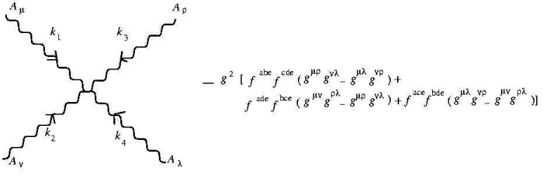
Interaction of Four Fluids System Dynamics
Following the same procedure as done in Sec. 3.2.1, we obtain
−iM4 =−g2
fabefcde gµρgνλ−gµλgνρ
for 4-point amplitude. Then, the squared amplitude becomes,
|M4|2 = g4
fabefcde gµρgνλ
−gµλgνρ
+
fadefbce gµνgρλ
−gµρgνλ
+facefbde gµλgνρ
−gµνgρλ
−gµα+
k1µk1α
m2
1 −
gν β +
k2νk2β
m2 2
−gργ+
k3ρk3γ
m2
3 −
gλσ+
k4λk4σ
m2 4
fabefcde gαγgβσ
−gασgβδ
+
fadefbce gαβgγσ −gαγgβσ
+facefbde gασgβγ−gαβgγσ
(d1 2 |~v1|
2
+V1)2− |~v1|2 (
d2
2|~v2|
2
+V2)2− |~v2|2
(d3 2 |~v3|
2+V
3)2− |~v3|2 (
d4
2|~v4|
2+V
4)2− |~v4|2
+2fabefcdefacefbde
the following relations hold,
ki·ki = m2i =ρ2iV2 ,
k1·k2 =
1
4ρ1v1ρ2v2(v1v2−4cosθ)V
2 ,
k1·k3 =
1
4ρ1v1ρ3v3(v1v3−4cosα)V
2 ,
k1·k4 = −
1 4(4ρ
2
1+ρ1v1ρ2v2(v1v2−4cosθ) +ρ1v1ρ3v3(v1v3−4cosα))V2 ,
k2·k3 = −
1 4 2(ρ
2 1+ρ
2 2+ρ
2 3−ρ
2
4) +ρ1v1ρ2v2(v1v2−4cosθ)
+ρ1v1ρ3v3(v1v3−4cosα))V2 ,
k2·k4 = −
1 4(2(ρ
2
1+ρ23−ρ22−ρ24) +ρ1v1ρ3v3(v1v3−4cosα))V2 ,
k3·k4 = −
1 4(2(ρ
2 1+ρ
2 2−ρ
2 3−ρ
2
Chapter 4
Discussion and conclusion
In this chapter we will describe an idea about application of the theory, i.e.the inter-actions of three or four fluids. Application of this theory can be used to show describe
the observable in a meeting point of river and sea. This means we can model, for
instance the turbuilence, at the point as one fluid coming from the river and the other
two fluids fields scattered away to the sea.
The application of 4-point scattering is much wider [9]. This can be used to deal with turbulence in any fluid system, nebula for cosmology, dynamics of nano-crystal
and so on. In all cases we can model all appropriate observables as a result of scattering
of 4 homogeneous fields coming into a point.
Finally we have shown that interaction of multi fluids system which is localized
on one fixed point could be counted based on gauge field theory. Further, there is a
special characteristic in the 3- and 4-point interactions. In the case of 3-point there is
no angle dependence at all, while in 4-point case the amplitude depends on two angles
Appendix A
Massive vector polarization
In the case of massive vector particle, the wave equation for a particle of mass M for a bosonic fieldAµ is written as [6],
(gν µ(2+M2)−∂ν∂µ)Aµ= 0, (A.1)
We can determine the inverse of the momentum space operator by solving
(gν µ(−k2+M2) +kνkµ)−1 =δλµ(Ag νλ
+Bkλkν), (A.2)
forAand B. The propagator, which is the quantity in brackets on the right-hand side of (A.2) multiplied by i, is found to be,
i(gν µ+kνkµ/M2)
k2 −M2 . (A.3)
We can show that the numerator is the sum over the spin states of the massive particle when it is taken on-shell,i.e.k2 =M2. We first take the divergence,∂
ν of (A.1), which
makes cancellation to find
M2∂µA
µ = 0 that is, ∂µAµ= 0, (A.4)
Thus, for a massive vector particle, we have no choice but to take∂µA
µ= 0. We should
remark that it is not a gauge condition. As a consequence, the equation is reduced to
be,
(2+M2)Aµ= 0, (A.5)
with free-particle solutions,
Aµ =ǫµe−ik·x with ǫµ=
d
2|~v|
2
−V,−~v
The condition in Eq. (A.1) demands,
kµǫ
µ = 0, (A.7)
which reduces the number of independent polarization vector from four to three in a
covariant fashion. For a vector particle of mass M, energy E and momentum ~k along the z−axis, the states of helicities λ can be described by polarization vectors
ǫλ=±1 =
∓(0,1√,±i,0)
2
d
2|~v|
2
−V,−~v
,
ǫλ=0 = (|k|,0,0, E)
M
d
2|~v|
2
−V,−~v
. (A.8)
Therefore the completeness relation is,
X
λ
ǫ뵆ǫ λ ν =
−gµν +
kµkν
M2
d
2|~v|
2
−V
2
− |~v|2
!
, (A.9)
Appendix B
Three points amplitude calculation
|M3|2 = g2(fabc)2
h
gµν(k
1−k2)ρ+gνρ(k2−k3)µ+gµρ(k3−k1)ν
i
(−gµα+
k1µk1α
m2 1
)(−gν β +
k2νk2β
m2 2
)(−gργ+
k3ρk3γ
m2 3
)
h
gαβ(k1−k2)γ+gβγ(k2−k3)α+gαγ(k3 −k1)β
i
(d1 2|v~1|
2
+V1)2− |v~1|2
(d2 2 |v~2|
2
+V2)2− |v~2|2
(d3 2|v~3|
2
+V3)2− |v~3|2
= g2(fabc)2[left
×(1)×(2)×(3)×right×scalar] = g2(fabc)2[left
×(1)×(2)×(3)×(A+B+C)×scalar] (B.1)
left =hgµν(k
1−k2)ρ+gνρ(k2−k3)µ+gµρ(k3−k1)ν
i
(B.2)
(1) = (−gµα+
k1µk1α
m2 1
); (2) = (−gν β +
k2νk2β
m2 2
); (3) = (−gργ +
k3ρk3γ
m2 3
) (B.3)
right = (A+B+C) =hgαβ(k
1−k2)γ+gβγ(k2−k3)α+gαγ(k3−k1)β
i
(B.4)
scalar =(d1 2 |v~1|
2
+V1)2−|v~1|2
(d2 2|v~2|
2
+V2)2−|v~2|2
(d3 2|v~3|
2
+V3)2−|v~3|2
left×(1)×(2)×(3)×(A) =
h
−(k1−k2)2−(k1−k2)·(k2−k3)−(k1−k2)·(k3−k1)
+k
2
1(k1−k2)2
m2 1
+ k1·(k1−k2)k1·(k2−k3)
m2 1
+k1·(k1−k2)k1·(k3−k1)
m2 1
+k
2
2(k1−k2)2
m2 2
+ k2·(k1−k2)k2·(k2−k3)
m2 2
+k2·(k1−k2)k2·(k3−k1)
m2 2
+(k3·(k1−k2))
2
m2 3
+k3·(k1−k2)k3·(k2−k3)
m2 3
+k3·(k1−k2)k3·(k3−k1)
m2 3
−(k1·k2)
2(k
1−k2)2
m2 1m22
−k1·k2k1·(k2−k3)k2·(k1−k2) m2
1m22
−k1·k2k2·(k3m−2k1)k1·(k1−k2)
1m22 −
k2
1(k3·(k1−k2))2
m2 1m23
−k1·k3k1·(k2m−2k3)k3·(k1−k2)
1m23 −
k1·k3k1·(k3−k1)k3·(k1−k2)
m2 1m23
−k
2
2k3·(k1−k2)2
m2
2m23 −
k2·k3k2·(k2−k3)k3·(k1−k2)
m2 2m23
−k2·k3k2·(k3m−2k1)k3·(k1−k2) 2m23
+ (k1·k2)
2(k
3·(k1−k2))2
m2 1m22m23
+k1·k2k2·k3k1·(k2−k3)k3 ·(k1 −k2)
m2 1m22m23
+ k1·k2k1·k3k2·(k3−k1)k3·(k1−k2)
m2 1m22m23
i
left×(1)×(2)×(3)×(B) =
h
−(k1−k2)·(k2−k3)−(k2−k3)2−(k3−k1)·(k2−k3)
+k1 ·(k1 −k2)k1·(k2−k3)
m2 1
+(k1·(k2−k3))
2
m2 1
+k1·(k2−k3)k1·(k3−k1)
m2 1
+k2 ·(k1 −k2)k2·(k2−k3)
m2 2
+k
2
2(k2·(k2−k3))2
m2 2
+k2·(k2−k3)k2·(k3−k1)
m2 2
+k3 ·(k1 −k2)k3·(k2−k3)
m2 3
+k
2
3(k2−k3)2
m2 3
+k3·(k2−k3)k3·(k3−k1)
m2 3
−k1·k2k1·(k2−k3)k2 ·(k1 −k2) m2
1m22
− k
2
2(k1·(k2−k3))2
m2 1m22
−k1·k2k1·(k2m−2k3)k2 ·(k3 −k1)
1m22 −
k1·k3k1 ·(k2−k3)k3·(k1−k2)
m2 1m23
−k
2
3(k1 ·(k2 −k3))2
m2
1m23 −
k1·k3k1·(k2−k3)k3·(k3−k1)
m2 1m23
−k2·k3k2·(k2m−2k3)k3 ·(k1 −k2)
2m23 −
(k2·k3)2(k2−k3)2
m2 2m23
−k2·k3k2·(k3m−2k1)k3 ·(k2 −k3) 2m23
+ k1·k2k2·k3k1·(k2−k3)k3·(k1−k2)
m2 1m22m23
+(k1·(k2−k3))
2(k 2·k3)2
m2 1m22m23
+ k1·k3k2·k3k1·(k2−k3k2·(k3−k1))
m2 1m22m23
i
left×(1)×(2)×(3)×(C) =
h
−(k1−k2)·(k3−k1)−(k2−k3)·(k3−k1)−(k3−k1)2
+k1·(k1−k2)k1·(k3−k1)
m2 1
+k1·(k2−k3)k1·(k3−k1)
m2 1
+k
2
1(k3−k1)2
m2 1
+k2·(k1−k2)k2·(k3−k1)
m2 2
+k2·(k2−k3)k2·(k3−k1)
m2 2
+(k2·(k3−k1))
2
m2 2
+k3·(k1−k2)k3·(k3−k1)
m2 3
+k3·(k2−k3)k3·(k3−k1)
m2 3
+k
2
3(k1−k2)2
m2 3
−k1·k2k1·(k1m−2k2)k2·(k3−k1)
1m22 −
k1·k2k1·(k2−k3)k2·(k3−k1)
m2 1m22
−k
2
1(k2·(k3−k1))2
m2
1m22 −
k1 ·k3k1·(k3−k1)k3·(k1−k2)
m2 1m23
−k1·k3k1·(k2m−2k3)k3·(k3−k1)
1m23 −
(k1·k3)2(k3 −k1)2
m2 1m23
−k2·k3k2·(k3m−2k1)k3·(k1−k2)
2m23 −
k2·k3k2·(k3−k1)k3·(k2−k3)
m2 2m23
−k
2
3k2·(k3−k1)2
m2 2m23
+k1·k2k1·k3k2·(k3−k1)k3·(k1−k2)
m2 1m22m23
+k1·k3k2·k3k1·(k2−k3)k2·(k3−k1)
m2 1m22m23
+(k1·k3)
2(k
2·(k3−k1))2
m2 1m22m23
i
+(k2·k3)
2(k
1·(k2−k3))2
m2 1m22m23
+ 2k1·k2k1·k3k2·(k3−k1)k3·(k1−k2)
m2 1m22m23
+(k1·k3)
2(k
2·(k3−k1))2
m2 1m22m23
+ 2k1·k3k2·k3k1·(k2−k3)k2·(k3−k1)
m2 1m22m23
i
Appendix C
Four points amplitude calculation
|M4|2 = g4
fabefcde gµρgνλ
−gµλgνρ
+
fadefbce gµνgρλ
−gµρgνλ
+facefbde gµλgνρ
−gµνgρλ
−gµα+
k1µk1α
m2
1 −
gν β+
k2νk2β
m2 2
−gργ+
k3ρk3γ
m2
3 −
gλσ+
k4λk4σ
m2 4
fabefcde gαγgβσ
−gασgβδ
+
fadefbce gαβgγσ −gαγgβσ
+facefbde gασgβγ−gαβgγσ
(d1 2 |~v1|
2+V
1)2− |~v1|2 (
d2
2|~v2|
2+V
2)2− |~v2|2
(d3 2 |~v3|
2+V
3)2− |~v3|2 (
d4
2|~v4|
2+V
4)2− |~v4|2
= g4[left
×(1)×(2)×(3)×(4)×right×scalar]
= g4[left×(1)×(2)×(3)×(4)×(A+B +C)×scalar]
(C.1)
left =
fabefcde gµρgνλ−gµλgνρ
+
fadefbce gµνgρλ
−gµρgνλ
+facefbde gµλgνρ
−gµνgρλ
+k1·k1(k2·k3)
2
−k1·k2k1·k3k2·k3
m2 1m22m23
+k2·k2(k1·k4)
2
−k1·k2k1·k4k2·k4
m2 1m22m24
+k3·k3(k1·k4)
2
−k1·k3k1·k4k3·k4
m2 1m23m24
+k4·k4(k2·k3)
2
−k2·k3k2·k4k3·k4
m2 2m23m24
+(k1·k3k2·k4−k1·k4k2·k3)(k1·k4k2·k3−k1·k2k3·k4)
m2
1m22m23m24
+k4·k4(k1·k2)
2
−k1·k2k1·k4k2·k4
m2 1m22m24
+k1·k1(k3·k4)
2
−k1·k3k1·k4k3·k4
m2 1m23m24
+k2·k2(k3·k4)
2
−k2·k3k2·k4k3·k4
m2 2m23m24
+(k1·k4k2·k3−k1·k2k3·k4)(k1·k2k3·k4−k1·k3k2·k4)
m2
1m22m23m24
+2k1·k2k1·k3k2·k3−(k1·k1(k2·k3)
2+k
3·k3(k1·k2)2)
m2 1m22m23
+2k1·k2k1·k4k2·k4−(k2·k2(k1·k4)
2+k
4·k4(k1·k2)2)
m2 1m22m24
+2k1·k3k1·k4k3·k4−(k3·k3(k1·k4)
2+k
1·k1(k3·k4)2)
m2 1m23m24
+2k2·k3k2·k4k3·k4−(k2·k2(k2·k4)
2+k
4·k4(k2·k3)2)
m2 2m23m24
+(k1·k2k3·k4)
2+ (k
1·k4k2·k3)2−2(k1·k2k3·k4)(k1·k4k2·k3)
m2
1m22m23m24
+2fadefbcefacefbde
(k1·k3)2−k1·k1k3·k3
m2 1m23
+(k1·k4)
2
−k1·k1k4·k4
m2 1m24
+(k2·k3)
2−k
2·k2k3·k3
m2 2m23
+ (k2·k4)
2−k
2·k2k4·k4
m2 2m24
+k3·k3(k1·k2)
2−k
1·k2k1·k3k2·k3
m2 1m22m23
+k4·k4(k1·k2)
2−k
1·k2k1·k4k2·k4
m2 1m22m24
+k1·k1(k3·k4)
2−k
1·k3k1·k4k3·k4
m2 1m23m24
+k2·k2(k3·k4)
2−k
2·k3k2·k4k3·k4
m2 2m23m24
+(k1·k4k2·k3−k1·k2k3·k4)(k1·k2k3·k4−k1·k3k2·k4)
m2
1m22m23m24
References
[1] A. Sulaiman, Master Theses at Department of Physics, University of Indonesia
(2005) ;
A. Sulaiman and L.T. Handoko,in preparation.
[2] M.V. Altaisky and J.C. Bowman, Acta Phys. Pol. (in press);
A.C.R. Mendes, C. Neves, W. Oliveira and F.I. Takakura, Brazilian J. Phys. 33
(2003) 346;
P. Lynch,Lecture Note : Hamiltonian Methods for Geophysical Fluid Dynamics -An Introduction (2002).
[3] A. Grauel and W.H. Steeb, Int. J. Theor. Phys. 24 (1985) 255.
[4] B. Bistrovick, R. Jackiw, H. Li and V.P. Nair, Phys.Rev. D67 (2003) 025013; T. Kambe,Fluid Dyn. Res. 32 (2003) 192;
R. Jackiw, Proc. of Renormalization Group and Anomalies in Gravity and Cos-mology, Ouro Preto, Brazil (2003).
[5] For example, see : T.P. Cheng and L.F. Li, Gauge theory of elementary particle physics, Oxford Science Publications (1991).
[6] For example, see : L.H. Ryder, Quantum Field Theory, Cambridge University Press (1985).
[7] For example, see : F. Stancu, Group Theory in Subnuclear Physics, Oxford Science Publications (1996).
[8] M.K. Verma, Int. J. Mod. Phy. B15 2001 3419.