Separate-activation models with variable
base times: Testability and checking
of cross-channel dependency
ROLF ULRICH and MARKUS GIRAYPsychologisches lnstitut der Universitas Tublngen, Tabingen, Federal Republic of Germany
Ifa subject is required to respond to either of two different target signals, reaction times (RTs) are especially fast when both target signals are presented. Separate-activation models can ac-count for this finding. This model class assumes that each target signal is detected in a different channel and that the detection time of each channel is a random variable.Iftwo different target signals are presented, RT is simply the lesser of the two detection times. Cumulative distribu-tion funcdistribu-tions of RTs are commonly used to test channel independence or, if channel indepen-dence is rejected, to evaluate the detection-time correlation. The present paper shows that it is important to consider the variability of the base time for all processes after the response has been decided on but before it has actually been carried out. It is shown that this variability in-fluences the determination of the detection-time correlation. In addition, it is shown that Miller's (1982)test of separate-activation models versus coactivation models can also be applied to models with variable base times.
In many tasks, human observers monitor two distin-guishable sources for a signal requiring a quick response. For example, in a bimodal detection task, the observer must respond as soon as a signal is presented on either of two modalities, say, vision and audition. On signal trials, only one signal (e.g., a tone or a flash) is presented, whereas on redundant-signal trials, both signals are presented simultaneously. Performance is studied in such a task by measuring the time (RT) between stimulation onset and response. The common finding is that RT is shorter for redundant-signal trials. This phenomenon has been called the "redundant signal effect" (Kinchla, 1974). Miller (1982) has recently distinguished two model classes to explain the redundant-signal effect: the separate-activation and the coseparate-activation models. Separate-separate-activation models assume that the two signals are processed simul-taneously within different channels and that each chan-nel produces a separate activation (cf. Meijers & Eijk-man, 1977; Raab, 1962). The response is initiated as soon as an activation level is exceededineither channel. In con-trast to separate-activation models, coactivation models assume that the signals on the different channels produce a combined activation, and that the response is initiated as soon as this combined activation exceeds a criterion level.
Miller (1982) proposed a general test for the class of separate-activation models. In short, he has shown that
We thank Hans Colonius, the Editor, Wilhelm Glaser, Dominic Mas-saro, two anonymous reviewers, and Dirk Vorberg for helpful com-ments on an earlier draft of this paper. Some results presented here were reported at the 25. Tagung experimentell arbeitender Psychologen, Ham-burg, 1983. Requests for reprints should be sent to Rolf Ulrich, Psy-chologisches Institut, Universitiit Tiibingen, Friedrichstrasse 21, 7400 Tiibingen, Federal Republic of Germany.
the inequality Gx(t)
+
Gy(t) セ Gn{t)-whereG(t)is the probability that a response has been made by timet, and X,Y,andXYrefer to conditions with a single-target sig-nal on channel Cs, a single-target signal on channelCy,and signals on both channels Cxand Cy-must be satis-fied for all values oftif separate-activation models hold. A violation of this inequality supports coactivation models and rejects separate-activation models.
Ifthe data satisfy the above inequality, and hence are consistent with the prediction of the separate-activation model, it is worthwhile investigating what type of separate-activation model might be consistent with the results obtained. In particular, recent papers have been concerned with the question of whether the detection times of the two channels are independent (Miller, 1982; Meijers & Eijkrnan, 1977), and, if independency is re-jected, whether they are positively or negatively correlated (Grice, Canham, & Boroughs, 1984; van der Heijden, Schreuder, Maris,& Neerincx, 1984). The baseline for this test rests on the following equality:
m(t) = Gx(t)+Gy(t) - Gx(t)*Gy(t), (1) wherem(t)denotes the predicted cumulative distribution functions (CDF) for redundant trials if the detection times are independent. Hence, ifm(t) and the observed CDF Gn{t) coincide, then it is concluded that the detection times are independent (Grice, Canham, & Boroughs, 1984; Meijers& Eijkrnan, 1977; Miller, 1982; van der Heiden et al., 1984). Grice, Canham, & Boroughs (1984) have even suggested a method to estimate the correlation of the detection times. In essence, this method yields a negative correlation ifGn{t)
>
m(t)and a positive corre-lation if Gn{t)<
m(t).The present work extends the test of Miller (1982). We
proceed from the additional assumption of a variable base time for all processes after the response has been decided on but before it has actually been carried out (e.g., mo-tor response times).Itwill be demonstrated that the varia-bility of the base time influences the outcome of tests us-ing Equality 1.
In addition it is shown that Miller's inequality can also beapplied to separate-activation models with variable base times. We also provide a lower bound forG;o{t).IfG;o{t)
falls short of this lower bound, then the whole class of separate-activation models has to be rejected.
SEPARATE-ACTIVATION MODELS WITH VARIABLE BASE TIMES
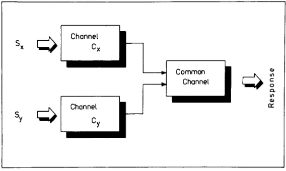
Figure I shows the basic structure of the generalized separate-activation model. The model assumes two chan-nels, Cx and Cy , operating in parallel. Each channel is
linked with one and only one source (e.g., visual or au-ditoryュッセ。ャゥセゥ・ウIN Each channel detects the relevant sig-nal occurnngInthe corresponding source. The two
chan-nels, C»andCy , run into a final one, called the common
channel. The common channel summarizes all the stages that follow stimulus detection. As soon as processing of the common channel ends, the subject's response occurs. Let X(Y)denote the detection time of target stimulus Sx(Sy) in channel
C«
(Cy). X and Yare assumed to be random variables which might be negatively or positively correlated, or be independent. The random variable Bdenotes the processing time (base time) of the common channel. According to the assumptions outlined, the RT forウゥョァセ・ signal trials is given by RTx=X
+
Bif only sig-nal SX IS presented, and by RTy=Y+
B if onlyS«
is presented. RTxydenotes the reaction time when both sig-nals。イセ presented, and is given byRTxy=min(X,y)+B. The minimum of X and Yis denoted by min(X,Y),which,stated in other terms, is the interim between onset of sig-nals and initiation of the common channel. Note that min(X,Y)is again a random variable. Since the mean of min(X,Y)must be smaller than or equal to either mean
of X and Y,the separate-activation model predicts faster
RTs, on average, for redundant signal trials than for each type of single-target trials.
Theorem 1:Let Gxy(t), Gx(t),and Gy(t) be the (ob-servable) CDFs of Rxy,
s..
ande;
respectively.If
the separate-activation model outlined aboveistrue, then theヲセャャッキゥョァ inequality must holdfor all values oft
irrespec-tive ofwhether or not the detection times Xand Yare cor-related (positively or negatively);
Gx(t)+Gy(t) セ Gxy(t) セ max[Gx(t),Gy(t)]. (2)
(The proof ofInequality 2 is contained in Appendix A. I) Inequality 2 defines an upper and a lower bound for
Gxy(t), and max[Gx(t),GY(t)] is the maximum value of the two CDFs Gx(t) andGy(t) at timet. Ifthe observed
G0t).isless than this maximum value, then all separate-activation models have to be rejected. This lower bound has already been utilized by Grice, Canham, and Gwynne (1984, pp. 568-569) in order to evaluate distraction ef-セ・」エウ in redundant target trials. The left side of Inequal-tty 2 puts an upper bound forGxy(t). IfGxy(t)is greater エィ。セ エセ・ sum of Gx(t) and Gy(t), then all separate-acuvanon models can be ruled out.Itshould be stressed that this test must hold (1) whether or not X and Yare
dependent, (2) whether or not the base-time variance is large, and (3) whether or not the detection times are cor-related with the base-time B; for example, there is some
・vゥ、・ョ」セ that .detectionand motor times are positively
cor-related Ina simple RT task (Ulrich& Stapf, 1984). The
left ウセ、・ ofセョ・アオ。ャゥエケ 2 agrees with Miller's (1982)
in-equality. ThIS makes it certain that Miller's inequality can also be applied to separate-activation models with vari-able base times.
What canbesaid aboutG;o{t)if the two detection times
X.
and Yare independent? The following corollary pro-vides an answer.Corollary:
If
the processing times X, Y, and Bare stochastically independent variables, then for all values t, the inequalityChannel
Cx セ
--
Common,---+ Channel
Channel
-Cy
[image:2.549.131.415.524.694.2]Gx(t)+Gy(t)-Gx(t)
*
Gy(t) 2= Gxit) (3)must hold. (The proof is contained in Appendix B.) Inequality 3 puts an upper limit on the observedGxit)
inthe case of independent detection times.Ifthe observed CDFsGx(t), Gy(t),andGxy(t)violate Inequality 3, then all independent-channels-separate-activation models can be rejected.
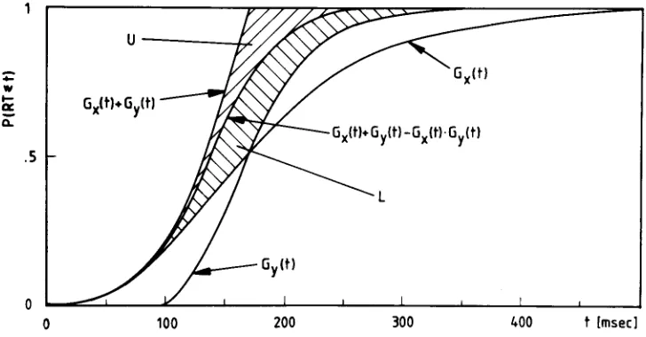
Figure 2 summarizes the above testable predictions for fictitious data. This figure shows two hatched regions, L (lower region) and U (upper region). U is bounded above by Gx(t)
+
Gy(t) and bounded below byGx(t)
+
Gy(t) -Gx(t)*
Gy(t),whereas L is bounded above by Gx(t)+GY(t)-Gx(t)*
Gy(t) and bounded below by max [Gx(t),Gy(t»). For all separate-activation models, the observedGxit)must be placed anywhere within U and/or L.Ifthe processing times are assumed to be independent, then Gxit) must be placed anywhere within regionL.ILLUSTRATING THE TESTS BY MONTE-CARLO SIMULATIONS
We conducted extensive simulationsdesigned to demon-strate the effects of the base-time variance on the empiri-cal determination of the detection-time correlation. In this simulation, it is assumed that X, Y, andB are normally distributed random variables. Approximate normally dis-tributed random numbers can be generated by using the method proposed by Box and Muller (1958), as shown by Equation 4:
Z = [-2
*
log(U1)l5*
cos(2*
1f*
U2 ) , (4)where Z is a normally distributed random deviate with zero mean and unit variance, andU1andU2are
indepen-dent random variables between 0 and I from a rectangu-lar distribution.
LetZI andZ2 be a pair of normal deviates generated by using Equation 4. Then the two random numbers
D1=ZIandD2 = corr
*
ZI+
(l r-corr")"*
Z2representa pair of deviates from a bivariate normal distribution with zero means, unit variances, and correlation coefficient corr(cf, Abramowitz&Stegun, 1972, p. 953). Each devi-ateD,ofthe pair(D1>D2 )can be linearly transformed by
usingT, = SDi
*
Di+
M, to obtain a normal distributedrandom number
To
with meanMi and standard deviation SDi , i= 1,2. The correlation coefficient between T1andT2equals corr, since any linear transformation of random
variables does not change their correlation.
Ten thousand trials were used to simulate the CDF of RTxy •In each trial, the following steps were performed: (I) A pair of correlated detection times X and Ywere generated, as outlined above, with means
M»
andMyand standard deviationsSDxandSDy , respectively. (2) Thesmaller value of X and Ywas determined; let S denote this minimum. (3) A normal distributed base-timeBwith meanMBand standard deviationSDBwas generated. (4) S
and B were added to produce RTxy •
The CDFs of RTx and RTywere obtained in a similar fashion. For example, to simulate RTxone has to gener-ate X andBin each trial and add these two random num-bers. Ten thousand trials were used to simulateGx(t), and a further 10,000 trials were used for Gy(t).
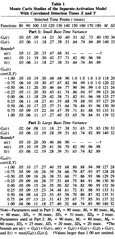
Table I summarizes the results for several simulations with different model parameters. A small base-time vari-ance was used for all simulations in Part 1 of Table 1, whereas a large base-time variance was used for simula-tions in Part 2. The same means,Mx, My,andMB , were
used for all simulations in Table 1. However, one set of standard deviations (SDx, SDy, SDB ) was used for Part 1,
and a different set was used for Part 2. The standard devi-ations in each part were adjusted in such a way that, for ease of comparison and tabular presentation, the
result-t Imsecl 400
300 200
100
o
o
u----...J...£
.5 :;;
w
[image:3.549.93.457.473.663.2]Ii
Gx(t)+ Gyltl Q.Selected Time Pointst(msec)
.05 .Il .20 .33 .47 .68 .91 -t
[image:4.549.44.270.64.532.2].05 .Il .19 .30 .42 .57 .71 .82 .90 .96 .98 .03 .06 .Il .18 .27 .38 .51 .64 .74 .84 .89
Table 1
Monte Carlo Studies of the Separate-Activation Model With Correlated Detection Times X andY
Functions 80 90 100 IlO 120 130 140 150 160 170 180 M SD Part 1:Small Base-Time Variance
Gx(t) .03 .05 .09 .14 .21 .30 .40 .51 .62 .73 .80 150 36 G,.(t) .03 .06 .Il .18 .27 .38 .51 .64 .74 .84 .89 140 32
The obtained pattern of simulated RTs agrees fairly well with the pattern of results in a real experimental condi-tion. "Statistical facilitation" (Rabb, 1962) is also ob-tained for this generalized version of the separate-activation model: both means RTx and RTyare always
greater than the corresponding mean of RTxy• One can
observe less "statistical facilitation" in the case oflarge base-time variance.
Detection-time correlation had a profound effect on
Gxy(t). In both parts of Table 1,Gxy(t) decreased with
increasing corr(X,Y). For example, we obtained Gn-(140)
=
0.90 for corr(X,Y)=
-1 in Part 1. As corr(X, Y) increases, Gn-(140) decreases to 0.53 for corr(X, Y)= 1. Increasing corr(X, Y) also increases the mean and the standard deviation of RTxy•Consider now the two boundsu(t)andl(t). According to Theorem 1, allGn-{t)s must be bounded above byu(t)
and below byl(t). As one can see, the resulting regions in Parts 1 and 2 are quite narrow, suggesting a powerful test of the separate-activation model. Table 1 shows that
allGn-{t)s fall within this specified region. This test does
not depend on the magnitude of the base-time variance. The variance of the base time poses problems for a re-cent suggestion and application of a method to estimate the detection-time correlation (Grice, Canham, & Boroughs, 1984, p. 452; van der Heijden et al., 1984). Grice, Canham, & Boroughs suggested constructing a fourfold table from which a phi coefficient or tetrachoric correlation might be computed using the CDFs of RTx, RTy, and RTxy. The proportions of responding and not
responding to the two types of signals on single signal trials provide estimates for the marginals of the table. The proportion of not respondingwhen both stimuliare present determines one cell of the table. Since the table has only one degree of freedom, the remaining three cells can be filled.
We will illustrate this method using the data of Table 1. For example, consider the time point t
=
150 msec inPart 1. A value of 0.94 is obtained for Gn-(150) and corr(X, Y) = -0.75. The corresponding values for Gx(l50) and Gy(150) are 0.51 and 0.64, respectively. Now one should useGn-{t)to compute the desired propor-tionP(RTx セ 150and RTy セ 150) = 1-Gn-(150) =
1-0.94
=
0.04 of not responding at timet=
150 msec when both stimuli are presented. This proportion is suffi-cient to complete the table for estimating the detection-time correlation. For the numerical example, one com-putes a phi coefficient of -0.49 and a tetrachoric corre-lation coefficient of -0.73. As one can see, the direc-tion and the magnitudeof the correladirec-tion coefficientsagree fairly well with the corresponding correlation coefficient used to generate the CDF.Let us now repeat the whole procedure for Part 2. A value of 0.79 was obtained for GxrtI50) at corr(X,Y)
=
-0.75. The corresponding values for Gx(l50) andGy(150)are 0.51 and 0.63, respectively. The same
com-putation as before yields a tetrachoric correlation of 0.19 and a phi coefficient of 0.12. This time the estimated coefficients agree neither in direction nor in magnitude .30 .48 .68 .90 1.0 1.0 1.0 1.0 1I8 20
.30 .47 .67 .82 .94 .99 1.0 1.0 120 22 .30 .46 .64 .77 .90 .96 .99 1.0 121 24 .30 .45 .61 .74 .86 .94 .97 .99 123 26 .29 .42 .58 .71 .82 .91 .96 .98 125 27 .27 .41 .55 .68 .79 .88 .93 .97 127 29 .25 .37 .51 .64 .76 .84 .91 .96 130 30 .22 .34 .47 .59 .71 .81 .88 .93 133 31 .17 .27 .40 .53 .65 .76 .84 .91 139 32
Bounds*
u(t) m(t) l(t) Gx,.(t)
corr(X,y)
-1.00 .05.10 .19 -0.75 .06.10 .19 -0.50 .06 .11 .20 -0.25 .05.Il .20 0.00 .00.Il .18 0.25 .00.Il .18 0.50 .06.10 .17 0.75 .05.09 .15 1.00 .03.06 .Il
Part 2:Large Base-Time Variance
Gx(t) .02 .04 .08 .Il .18 .27 .38 .51 .63 .75 .83 150 33
G,.(t) .03 .06 .12 .19 .28 .39 .51 .63 .74 .82 .89 140 32
Bounds*
u(t) .05 .10 .20 .30 .46 .66 .90 -t
m(t) .05 .10 .19 .29 .41 .56 .70 .82 .90 .96 .98
l(t) .03 .06 .12 .19 .28 .39 .51 .63 .74 .82 .89
Gx,.(t)
corr(X,y)
-1.00 .05 .10 .17 .27 .40 .55 .68 .80 .88 .94 .98 127 28 -0.75 .05 .09 .16 .26 .39 .54 .66 .79 .87 .93 .97 128 28 -0.50 .05 .09 .16 .26 .38 .53 .66 .77 .86 .93 .96 129 29 -0.25 .05 .09 .16 .26 .37 .51 .64 .75 .84 .91 .96 130 30 0.00 .05 .09 .15 .24 .35 .50 .62 .74 .82 .90 .95 132 30 0.25 .05 .09 .15 .23 .34 .48 .61 .72 .81 .88 .93 133 31 0.50 .04 .08 .14 .23 .33 .45 .58 .70 .80 .87 .92 135 31 0.75 .04 .07 .13 .21 .31 .43 .55 .67 .77 .85 .91 137 32 1.00 .04 .06 .Il .18 .27 .40 .52 .64 .74 .83 .90 140 32
Note-Parameters used in Part 1:Mx=90 msec,My=80msec,Ms
= 60msec, SDx = 36msec, SDy = 31msec, SDs = 2msec. Parameters usedin Part 2: Mx =90 msec, My =80msec, Ms =
60msec,SDx = 25rnsec,SDy= 20msec,SDs = 20msec. *The bounds areu(t)=Gx(t)+G,.(t),m(t) =Gx(t)+G,.(t)-G.(t)*G,.(t),
andl(t) = max[Gx(t),G,.(t)l. tValues larger than1.00are omitted.
ing CDFs of both parts had about equal spread and lo-cation.
Consider the different aspects within each of the two parts. The first two rows show the CDFs for RTx and RTr- These CDFs were used to calculate the three differ-ent bounds forGn-{t)according to Theorem 1 and the cor-rollary. These bounds appear beneath the CDFs of RTx and RTy. Then the subsequent rows show eight various
with the true detection-time correlation of-0.75.These computations show that the proposed method of Grice, Canham, and Boroughs (1984) for estimating the detection-time correlation works well if the base-time var-iance is very small; however, it leads to wrong estimates if the base-time variance is relatively large. The simula-tions with a high base-time variance reveal a systematic overestimation of the detection-time correlation coefficient actually used in the simulation. A mathematical explana-tion of this systematic bias is given in Appendix C.
This consideration may also help to clarify some difficulties concerning the explanation of recent results obtained in a simple letter-detection paradigm (van der Heijden et al., 1984). Subjects were required to perform a speeded response if a target letter was presented at either of two different locations. On single-target trials, only one letter was presented at either of two different locations, whereas in redundant target trials, two target letters were presented at both locations. Their results showed a clear redundant-signal effect, and the authors favored a separate-activation explanation after applying Miller's (1982) test. In a further analysis, the authors investigated the direction of the detection-time correlation with the method outlined above. The analysis revealed a "rather unexpected pattern" (van der Heijden et al., 1984, p. 582): The observed Gn{t) for redundant signal trials exceeds the base-linem(t)for small values oftbut falls short of this base line for intermediate and larger values oft. Hence, negative correlation coefficients were esti-mated for small values oft and positive ones were
esti-mated for larger values oft. Given our analysis, their results are consistent with negatively correlated detection times for all values oft, since Gn{t) may fall short of
m(t)if the detection times are negatively correlated, as Part 2 of Table 1 shows. That is, ifGn{t)falls short of
m(t),one cannot reject a negative detection-time
corre-lation. Clearly, this interpretation requires that the base-time variance be relatively large compared with the vari-ance of the detection-times. However, this requirement is not well supported empirically (Ulrich& Stapf, 1984; Wing & Kristofferson, 1973).
CONCLUSION
The present paper considered separate-activation models with variable base times. It was shown that Miller's (1982) upper boundGn{t) セ Gx(t)
+
Gy(t) could also be applied to check this more general model class against coactiva-tion models. In addicoactiva-tion, we provided a lower bound which may be used, for example, to reveal inhibitory ef-fects upon RT in redundant signal trials (cf. Ueno, 1977). The variability of the base time does not influence the out-come of these two tests.However, this variability influences the outcome of more specific questions regarding the dependence of the detection times: (1) It was shown that the base line,
Gx(t)+Gy(t)-GY(t)
*
Gx(t), usually used to checkin-dependence of the detection times, can be applied only
if one proceeds from a zero base-time variability. (2) Estimates of the detection-time correlation are in-fluenced by the magnitude of the base-time variability. In general, the detection-time correlation will be over-estimated if one applies the method suggested by Grice, Canham, and Boroughs (1984). The degree of overesti-mation depends largely on the magnitude of the base-time variability. Accurate estimates result with a zero base-time variability.
REFERENCES
ABRAMOWITZ, M.,&STEGUN,I.A. (1972). Handbook ofmathemati-cal functions with formulas. graphs. and mathematiofmathemati-cal tables. New York: Dover.
Box, G. E. P.,& MULLER, M. E. A. (1958). A note on the generation of random normal deviates. Annals of Mathematical Statistics,29, 610-613.
GRICE, G. R., CANHAM,L.,&BOROUGHS,J. M. (1984). Combination rule for redundant information in reaction time tasks with divided at-tention. Perception &Psychophysics,35, 451-463.
GRICE, G. R., CANHAM,L.,& GWYNNE,J. W. (1984). Absence of a redundant-signals effect in a reaction time task with divided atten-tion. Perception &Psychophysics,36, 565-570.
KINCHLA, R. (1974). Detecting target elements in multielement arrays: A confusability model. Perception& Psychophysics, IS, 149-158. MElJERS,L.M. M.,&EIJKMAN, E. G.J.(1977). Distributions ofsim-pie RT with single and double stimuli.Perception&Psychophysics,
22, 41-48.
MtLLER,J. (1982). Divided attention: Evidence for coactivation with redundant signals. Cognitive Psychology, 14, 247-279.
RAAB, D. H. (1962). Statistical facilitation of simple reaction time.
Trans-action of the New York Academy of Sciences, 24, 574-590. TOWNSEND, J. T., & ASHBY, F. G. (1983). Stochastic modeling of
elementary psychological processes. Cambridge: Cambridge Univer-sity Press.
UENO, T. (1977). Reaction time as a measure of temporal summation at suprathreshold levels. Vision Research,17, 227-232.
ULRICH, R.,& STAPF, K. H. (1984). A double response paradigm to study stimulus intensity effects upon the motor system.Perception &Psychophysics,36, 545-558.
VAN DER HEIJDEN, A. H. C., SCHREUDER, R., MARIS,L.,& NEERINCX, M. (1984). Some evidence for positively correlated separate activa-tion in a simple letter-detecactiva-tion task. Perception&Psychophysics,
36, 577-585.
WING, A. M.,& KRISTOFFERSON, A.B.(1973). Response delays and the timing of discrete motor responses.Perception&Psychophysics,
14, 5-12.
NOTE
1. The reader should note that the left-hand side of Inequality 2 is the identical inequality already proved by Miller (1982, p. 253). However, Miller (1982) did not explicitly state whether or not this ine-quality was also valid for separate-activation models with a variable base time. Hence, we tried to make certain that his inequality could also be applied to models with a variable base time.
APPENDIX A Proof of the Left-Hand Side of Inequality 2
Since theequationmin(X,Y)+B = min(X+B,Y+B) must hold, we can write
RTxy= min(X,y)
+
BGx,.(t)
= P(RTx ::S t)+P(RT y ::S t)-P(RTx ::S t and RTy ::S t).
Now we use Miller's (1982, p. 253) argumentation, P(RTx
::S tand RTy ::S t) セ 0, which yields the prediction
Gx,.(t) ::S P(RTx ::S t) + P(RTy ::St)
::SGx(t) + G,.(t).
The proof of the left-hand side of Inequality2is complete.
Proof of the Right-Hand Side of Inequality 2
IfGx,.(t) セ Gx(t) and Gxy(t) セ G,.(t)is true, thenGx,.(t) セ
max[Gx(t),G,.(t)]must also be true. Hence, we have to prove each of the two inequalities Gx,.(t)セ Gx(t)andGx,.(t) セ G,.(t)
separately. Take, for example, Gx,.(t) セ Gx(t):
Above we showed
Gx,.(t)
=
Gx(t)+G,.(t)-P(RTx ::S t and RTy::St), (AI) which can be rewritten, using conditional probability P(A and B) = P(AIB)P(B), asGx,-(t)
=
Gx(t)+G,.(t)-P(RTx ::S tIRTy ::St)G,.(t)= Gx(t)+G,.(t)[l-P(RTx::S tlRTy::S t)].
SinceP(RTx ::StIRTy::St)can maximallybeequal to one,
it follows that Gx,-(t) セ Gx(t) must be true.
In an analogous manner, one can prove thatGx,.(t) セ G,.(t)
if one substitutesP(RT y::S tIRTx ::St)Gx(t) for P(RTx ::S t
and RTy::St) in Equation A1.The proof is complete.
APPENDIX B
To simplify matters, we write S for min(X,Y). Thus, RTxy
equals the sumS+B; then the CDF ofRTxyis given by
Gxy(t)
=
P(S+B::St)=
II
!s(x)!B(y)dxdyx+ys/
(BI)
whereFs(t) and!B(t)are the CDF and the density function of Sand B, respectively. Since S is the minimum of X andY,
Fs(t) = P(X::st) + P(Y::s t) - P(X::st and Y::sr). It is assumed that X and Yare stochastically independent vari-ables; hence,
Fs(t) = Fx(t) + F,.(t) - Fx(t)F,.(t), (B2) whereFx(t)andF,.(t)are the CDFs of X and Y, respectively.
Inserting Equation B2 into Equation BI yields
iセfクHエMyIAィI、y
+I
セ
F,.(t-y)!h)dy - (Fx(t-Y)F,.(t- y)!8(Y)dy.The first two terms on the right side of the last expression are the convolution integrals (cf. Townsend&Ashby, 1983, pp. 30) of the sums X+Band Y+B, respectively. Therefore, we can rewrite the last expression
Gx,.(t) =
gクHエIKgLNHエIMiセfクHエMyIfLNHエMyIAィI、yN
(B3) The corollary states that the following inequality should hold if X and Yare independent:Gx(t)+G,.(t)- Gx(t)G,.(t) セ Gx,.(t).
Inserting EquationB3in the right-hand side, simplifying, and rewriting yields
I:Fx(t-Y)F,.(t-Y)!8(Y)dY-Gx(t)G,.(t)
セ
0iセfクHエMyIfLNHエMyIAィI、y
- [(FX(t-Y)!B(Y)dY] .
{AセfLNHエMyIAbHケI、y}
セ
O. (B4)This inequality is easily shown to be true. To this end, we de-fine two functions, hx(y)andh,.(y):
[
Fx(t-y) for y«:t, [F,.(t-y) for y<t,
hh)= h,.(y)=
o
otherwise 0 otherwise. We rewrite Equation B4, using the definitionshh)andh,.(y):!;
hx(y)h,.(y)!h)dy- [C
hh)!h)dY] .[C
h,.(y)!B(Y)dY]セ
O. Note that the integrals are expectations of the random variableshx(B)
*
h,.(B), hx(B),andh,.(B), respectively. (One should note that any function ofBmustbeagain a random variable.) Tak-ing this consideration into account yieldsE[hx(B)h,.(B)] - E[hx(B)] . E[h,.(B)] セ 0
cov[hx(B),h,.(B)] セ 0,
where the last expression is the covariance ofhx(B)andh,.(B).
Since bothhx(y)andh,.(y)decrease withY, it must always be true that the covariance ofhx(B)andh,.(B)is equal to or greater than zero. The proof is complete.
APPENDIX C
One outstanding result of the simulations is that the estimates of the detection-time correlations show a positive bias, that is, the estimates are always larger than the corresponding correla-tion coefficients used in the simulacorrela-tions. This effect is especially salient in the case of high base-time variance. This may be a little surprising, since, intuitively,one might expect that an added random variable simplyattenuateswhatever detection-timecorre-lation coefficient was used in the simudetection-timecorre-lation. Since this effect turns out to be systematic, a mathematical explanation of it may be helpful to correct one's intuition.
min(RTx,RT -) must hold, irrespective of whether or not X and Yarecorrelated and whether or not the variance ofBis large. This relation shows that RTxycan actuallybeconceived as the
minimum of RTx and RTy •Next, since the estimation proce-dure of Grice, Canham, and Boroughs (1984) utilizes RTs, the obtained estimates evaluate the correlation of RTx and RTy in
redundant signal trials instead of the desired correlation of X andY.Itis obvious, then, that corr(RTx,RTy)
>
corr(X,Y)if var(B)>
0, as the following mathematical analysis shows:To keep the analysis simple, we assume equal variances of X andY,that is, var(X)
=
var(Y). Now the correlation of RTx and RTy is given bycov(RTx, RTy) SD(RTx ) SD(RTy ) .
Since RTx
=
X+B, RTy=
Y+B, and var(X)=
var(y), we havecov(X+B,Y+B) corr(RTx,RTy ) = var(X+B) .
The numerator of the last expression can be rewritten by using the distributive property of covariances (see Ulrich & Stapf, 1984, p. 557) ascov(X+B,Y+B)
=
cov(X,y) + cov(X,B) + cov(B,y) + var(B). Since the base time,B, was uncorrelated with either detection time in the above simulations, we have cov(X+B,Y+B)=
cov(X,y) + var(B) and var(X+B)=
var(X) + var(B). Substituting these results into the last expression yields:cov(X,Y)+ var(B) corr(RTx,RTy) = var(X)+var(B)'
Since var(X)
>
0, we can divide the numerator and the denomi-nator of the above fraction by var(X), yieldingcorr(X,Y)+ var(B)/var(X)
corr(RTx,RTy ) = I+var(B)/var(X) . (Cl)
Itcanbeeasily shown, using Equation Cl ,that corr(RTx,RT-) increases with var(B) ifallother things are kept equal, and hence no attenuation of corr(X,Y)will result if the base-time variance increases.
Next we will show that corr(RTx,RT-) > corr(X,Y) if var(B)
>
0:corr(RTx, RTy )
>
corr(X,Y).Inserting Equation Cl for corr(RTx,RTy ) yields
corr(X,Y)+ var(B)/var(X)
1+ var(B)/var(X)
>
corr(X,Y).After rearrangement and cancellation, we arrive at corr(X,Y) < 1, showing that the assumed direction of the in-equality sign must hold.
In sum, the mathematical analysis shows that(1)corr(X,y) is overestimated if one utilizes RTs for its estimation and (2) that the degree of this bias depends on the relative magnitude of the base-time variance (cf. Equation Cl).
(Manuscript received June 18, 1985; revision accepted for publication April 14, 1986.)