DOI: 10.12928/TELKOMNIKA.v14i1.3540 684
Comparative Analysis of Spatial Decision Tree
Algorithms for Burned Area of Peatland in Rokan Hilir
Riau
Putri Thariqa1, Imas Sukaesih Sitanggang*2, Lailan Syaufina3 1,2
Department of Computer Science, Faculty of Natural Science and Mathematics, Bogor Agricultural University, Indonesia
3
Department of Silviculture, Faculty of Forestry, Bogor Agricultural University, Indonesia *Corresponding author, e-mail: [email protected], [email protected],
Abstract
Over one-year period (March 2013-March 2014), 58 percent of all detected hotspots in Indonesia are found in Riau Province. According to the data, Rokan Hilir shared the greatest number of hotspots, about 75% hotspots alert occur in peatland areas. This study applied spatial decision tree algorithms to classify classes before burned, burned and after burned from remote sensed data of peatland area in Kubu and Pasir Limau Kapas subdistrict, Rokan Hilir, Riau. The decision tree algorithm based on spatial autocorrelation is applied by involving Neigborhood Split Autocorrelation Ratio (NSAR) to the information gain of CART algorithm. This spatial decision tree classification method is compared to the conventional decision tree algorithms, namely, Classification and Regression Trees (CART), C5.0, and C4.5 algorithm. The experimental results showed that the C5.0 algorithm generate the most accurate classifier with the accuracy of 99.79%. The implementation of spatial decision tree algorithm successfully improves the accuracy of CART algorithm.
Keywords: classification, decision tree, peatland, spatial autocorrelation
Copyright © 2016 Universitas Ahmad Dahlan. All rights reserved.
1. Introduction
Fires in peatland/forest are very difficult to be handled than the fires that occurred in the area of non-peat. Peat fires (ground fire) difficult to detect because it can spread to the deeper or spread to more distant locations without being seen from the surface [1]. Processing of satellite images produced from remote sensing is able to provide convenience for stakeholders in monitoring the fire that has happened, is happening, and estimates the incidence of fires in the future. Additionally it can estimate the area burned and predicted environmental changes caused by the fire for a certain period [2].
One use of satellite image is to make the process of classification. There are several classification algorithms such as decision trees, Bayesian Networks, Naive Bayes, Maximum Likelihood and Minimum Distance. Some researches on satellite image classification have been carried out using decision tree algorithms. Sharma et al. [3] conducted a satellite image classification using the decision tree algorithm and compared with the ISODATA algorithm and maximum likelihood. The result shows that a decision tree has the best accuracy compared to other algorithms. The decision tree has proven to be an efficient algorithm for the classification of large datasets.
information about road networks, population census, buildings, and other geographic neighborhood details [5]. The different between spatial and non-spatial decision data is that in the spatial data, an object may have a significant influence on neighboring objects. Therefore, improvement of the non-spatial decision tree algorithm has been done by involving spatial relationships between two spatial objects [6].
The importance of spatial and autocorrelation aspect makes Jiang et al. [7] added autocorrelation aspect into a decision tree algorithm. Implementation of conventional decision tree algorithms including ID3, C4.5 and CART in the geographical classification implicitly assumes that data items are independent and ignores spatial autocorrelation effect. Thus, the classification result contains salt-n-pepper noise. To reduce the noise, autocorrelation aspects must be considered. Jiang et al. [7] conducted a classification using a spatial decision tree algorithm, which combined spatial autocorrelation as a measure of new formula of information gain. In the new formula of information gain had the most important parameter ( =0.26), this paramater is also applicable for the other areas. The study successfully reduced noise and obtained higher accuracy than the C4.5 algorithm. But, Jiang research only compared spatial decision tree with C4.5 algorithm and the autocorrelation was added to information gain from C4.5 algorithm. Jiang didn’t try to compare with other decision tree algorithm and didn’t try to use other information gain. Various algorithms including ID3, C4.5, CART, Random Forest had been used to classify satellite images, except the C5.0 algorithm that is still rarely used, because C5.0 algorithm is a new algorithm as the development of C4.5 algorithm.
This work applies the method of decision tree based spatial autocorrelation namely spatial decision tree (SDT) to classify peatland before burned, burned, and after burned in Kubu subdistrict and Pasir Limau Kapas subdistrict, Rokan Hilir, Riau Province. Parameter and autocorrelation was added to CART algorithm for this work, because SDT have a similar concept with CART algorithm. This work tried the other parameter for the best result. The results from the decision tree based spatial autocorrelation algorithm are compared with the other decision tree algorithm like CART algorithm, C5.0 algorithm and C4.5 algorithm. Comparison algorithm is done to determine whether the SDT is better than traditional decision tree algorithm. According to the comparison of the four algorithms, the best algorithm for classifying peat fire was analyzed. The results were expected to be used to calculate extent of the area in the classes of before burned, burned, and after burned.
2. Research Method
Study area in this research is peatland in Kubu subdistrict and Pasir Limau Kapas subdistrict, Rokan Hilir, Riau Province. This studied used remote sensing data, peatland map, and hotspots. Satellite images used were Landsat 7 in Rokan Hilir district, Riau Province which was taken from the USGS (United States Geological Survey). There were four images used that are images acuired in May, July, August, and November 2002. Peatland map 2002 in Riau was used to locate the peatland cover on the satellite image. The map of peatland that is represented in polygons was obtained from Wetlands International. The hotspots in July 2002 were obtained from MODIS Fire FIRMS / Hotspot, NASA / University of Maryland. Hotspots were used to determine the classes before burned, burned, and after burned.
2.1. Decision Tree based Spatial Autocorrelation
The decision tree method can automatically select the appropriate supporting attributes that iteratively split the given dataset into smaller groups according to the different values of these attributes [8]. The basic concept of the decision tree is to convert the data into a tree and decision rules. The decision tree consists of a root node at the top of the tree, the internal node which is a branch of the tree, and the leaf node which is the end of a tree branch.
Г′
Г (1)
Where Гi and Г’i are local gamma of sample i before and after split respectively. Spatial autocorrelation is often significant at local neighborhood level. Thus, we adopt the local gamma autocorrelation, formally defined as follows [7]:
Г ∑ , , ∑ , , (2)
Where i, j are sample indices; , , , are spatial similarity and class similarity, they are further represented by W-matrix , and indicator function , will have a value of 1 if it has the same class and is 0 if it has a different class; is count of homogeneous neighbors. NSAR values used in spatial information gain are NSAR value of all samples. NSAR value of all samples defined as follows [7]:
∑ (3)
Where i is the index of a sample, varying from 1 to m (m is the number of samples). From Equation (1), (2) and (3) spatial information gain is obtained as presented at following equation [7]:
SIG 1 α (4)
Where α is a balancing parameter.
2.2. Methodology
Analysis includes four major steps, namely, (1) image pre-processing, (2) determining classes of image, (3) distribution of training data and testing data and classification process, (4) evaluation and comparative analysis of classification results.
2.2.1. Image Pre-processing
The first preprocessing stage is georeferencing. Georeferencing produces raster maps which had the projected coordinate system UTM Zone 47 N with WGS84, meaning that Rokan Hilir is located at 47 N zone in the UTM (Universal Transverse Merctator) projection system with geospatial reference system of WGS84.
Combination red green blue (RGB) of a few bands causes images had different information. In this study, the combination of the image involved is band 7, band 4, and band 2. The band 7 is represented in red, the band 4 is represented in green, and the band 2 is represented in blue. In this band combination, vegetation area is shown by the green color, because the band 4 which had high reflectance of the vegetation represented by the green color. Band 7 is sensitive to radiation thus it allows detecting a heat source. Moreover, according to Wagtendonk et al. [9] uses of band 4 and band 7 of Landsat ETM+ is valid to detect the burn scars.
This study used satellite images of rokan Hilir that have peatland cover. Overlay and crop satellite images with maps of peat are necessary to get the image that has peatland cover. Overlaying was conducted to determine the areas of peatland cover, and cropping was carried out to take peatland area only. Satellite images with peatland cover still have a lot of clouds; therefore it was necessary to select a subset of image with clean of the cloud. The results of subset images include in Kubu subdistrict and Pasir Limau Kapas subdistrict, Rokan Hilir, Riau.
2.2.2. Determine Class of Image
2.2.3. Distribution of Training Data and Testing Data and Classification Process
Before the classification stage, the data were divided into several experimental groups using K-fold cross validation with k of 10. In which 9/10 data were used as training data and 1/10 data were used as testing data. Classification process was conducted using R software.
The decision tree based spatial autocorrelation algorithm using spatial information gain in Equation (4). This study uses several balance parameters (alpha) in equation (0.1, 0.14 and 0.26) of 0.1 because it result the best accuracy of the classiffier. Instead of using the entropy of C4.5 algorithm in the calculation of information gain as in Jiang et al. [7], this study used the gini gain value in CART algorithm. Here is the equation used to calculate the gini gain [10]:
1 ∑ (5)
, ∑ | || | (6)
Where is the probability of in the class , is the partition of S induced by the value of attribute A.
2.2.4. Evaluation and Comparative Analysis of Classification Results
Evaluation was conducted on accuracy, size of trees, and number of rules of the four algorithms. Accuracy was calculated using confusion matrix. Next, comparative analysis of classification outcomes used spatial decision tree based spatial autocorrelation algorithm, the CART algorithm, the C4.5 algorithm and the C5.0 algorithm.
3. Results and Analysis 3.1. Determine Class of Image
Buffers with radius 1 km were created for hotspots data. This radius of 1 km was used because the area for one hotspot in average is 2.58657 km, therefore the radius of the circle is 0.90737 km. This value is considered as the radius of a buffer for a hotspot. Outside the buffers, random points are generated as false alarm data [11]. Overlaying between buffer zone of hotspots and satellite image was useful to get information about the class before burned, burned, and after burned. Cropping process was performed to get a buffer area in the satellite image.
The buffer zone was converted into a digital number. The image in August that would be used for classification also converted into a digital number. In one pixel there were three digital numbers. A digital number was obtained from band 7, band 4, and band 2 because of composite process. Digital values derived from the buffer zone were matched with the digital values of the image in August. If those three digital values of the buffer zone equal to digital number of image in August, then the pixel has a buffer zone as the matched class. If in images acquired in August there are pixels that does not have a class or not equal with the pixels of the existing buffer zone, then the pixels are classified as a non peatland.
3.2. Evaluation and Comparative Analysis of Classification Results
which would improve the accuracy and discard the attributes that has less contribution or irrelevant [12].
Table 1. Classification comparison result
Algorithm Accuracy (%) Number of rules Size of tree
C4.5 98.89 1681 3362
C5.0 99.79 595 1603
CART 95.67 8 15
Spatial Decision Tree (SDT) 96.39 11 20
CART and the SDT algorithm create trees by using binary split. Binary split simplify the distribution criteria by considering all possible divided attributes, then choosing the best one. This situation causes on number of rules and size of tree in CART and SDT are lower than C4.5 and C5.0. The simplify rules that resulted from binary split has the lower accuracy compared with multisplit rules. Although, both CART and SDT used gini index, SDT has accuracy of 0.7% better than CART algorithm, because the SDT algorithm includes spatial autocorrelation aspect that considers neighbourhood value from every pixels inside information gain computing process.
The comparison of the four algorithms shows that the algorithm C5.0 had the best accuracy in multi-split criteria and algorithms SDT had the best accuracy in binary split criteria. Although the C5.0 algorithm has 3.4% better accuracy than the algorithms SDT, but it is not efficient. The efficiency of an algorithm is performed in term of the speed, scalability, and interpretation [13]. The speed of an algorithm was observed when the model is used to classify a new data. The rules are generated from the decision trees. The number of rules generated from C5.0 algorithm is greater than SDT algorithm with 595 rules and SDT algorithm only have 11 rules. The implementation of classification new data using C5.0 algorithm, may take longer time process. SDT algorithm will require shorter time because the number of rules generated is less than C5.0 algorithm. But, the accuracy resulted from SDT algorithm is smaller than those of C5.0 algorithm. Both of these algorithms satisfy the criteria of scalability because they were able to build a model that had a fairly good accuracy with a large number of data. C5.0 algorithm was more difficult to interpret, because it has a complex rules and trees. It differs from the SDT algorithm that was easy to understand because of the simpler rules and trees. The time complexity of the C4.5 algorithm and C5.0 algorithm is О(mn2),where m is the size of datasets and n is the number of attributes [14]. The time complexity of the algorithm CART and SDT which applied the concept of a binary tree is О(N log N) [15], where N is a number of attributes. CART and SDT algorithm had simpler complexity than C4.5 and C5.0 algorithm.
Li et al. [16] also compared decision tree algorithm in remote sensing. The accuracy of C4.5 algorithm was 0.866 and accuracy of CART algorithm was 0.857. C4.5 algorithm had a good accuracy, although CART algorithm has more training samples than C4.5. This shows the C4.5 algortihm is the best algorithm however the condition of the data. But the C4.5 algorithm was lost than the C5.0 algorithm, it can be proved on the results of this study were discussed in the paragraph above.
Table 2. Confusion matrix of classifier from C5.0 algorithm
Actual Prediction
Non-Peat Before Burned After Burned Burned
Non-Peat 327 0 3 0
Before Burned 0 81716 35 0
After Burned 2 5 9674 46
Burned 0 0 29 9393
Table 3. Confusion matrix of classifier from SDT algorithm
Actual Prediction
Non-Peat Before Burned After Burned Burned
Non-Peat 210 56 25 37
Before Burned 3 81284 434 0
After Burned 0 1059 7216 1466
Table 2 and Table 3 are confusion matrix derived from one experiment fold. Accuracy of the classifier from C5.0 algorithm in Table 2 is 99.88%, and the accuracy of the classifier from SDT algorithm in Table 3 is 96.47%. Confusion matrix obtain from the classification process using SDT algorithm showed that there are similarities between after burned class with burned class, and between after burned class with before burned class. Similarities between after burned class with before burned class occurred because condition of the land after burned has turn back into peatlands and the color became green again. The green color shows vegetation. Meanwhile the similarities between after burned class with burned class occurred because burned area still in the red color, red color shows burned area.
Figure 1. Image before classification
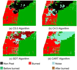
(a) C5.0 Algorithm (b) C4.5 Algorithm
(c) SDT Algorithm (d) CART Algorithm
Non Peat Burned Noise
Before burned After burned
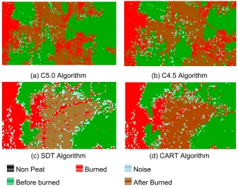
(a) C5.0 Algorithm (b) C4.5 Algorithm
(c) SDT Algorithm (d) CART Algorithm
Non Peat Burned Noise
Before burned After Burned
Figure 3. Image classification results were contaning noise around burned class and after burned class
The resulted of image classification will had salt-n-pepper noise. Noise salt-n-pepper is white dots or black contained in the image classification results. Noise arises because there is a class of misclassified. Figure 1 is image before classification process. In Figure 1 after burned class looks like noise because after burned area appear around burned area and they have small measure. Image that has the most noise is image resulted from CART algorithm, and SDT algorithm is able to reduce that noise. The most noise resulted around non peat class, burned class, and after burned class. Figure 2 are image resulted from C5.0, C4.5, SDT, and CART algorithm which has noise around non peat class. Figure 3 are image resulted from 4 algorithms which has noise in after burned class and burned class. The C5.0 algorithm had less noise, because this algorithm had the best accuracy.
Rules from SDT algorithm indicated that before burned class has band 4 value greater than the band 7 value, a burned class has band 7 value greater than the band 4 value, after burned class was in the middle value of the band, and the non-peat class has band 2 value greater than any other band. Here were 11 rules resulted from the SDT algorithm:
1. IF Band4 > 54 AND Band7 > 13 AND Band7 ≤ 51 THEN Before Burned 2. IF Band7 > 51 AND Band4 > 70 THEN Before Burned
3. IF Band4 > 54 AND Band7 ≤ 13 THEN Before Burned
4. IF Band4 ≤ 54 AND Band7 ≤ 41 AND Band2 ≤ 49 THEN Before Burned
5. IF Band4 > 54 AND Band7 > 51 AND Band4 ≤ 70 AND Band7 ≤ 79 THEN After Burned
6. IF Band7 > 41 AND Band4 ≤ 43 AND Band7 ≤ 54 THEN After Burned
7. IF Band4 ≤ 54 AND Band7 > 41 AND Band7 ≤ 66 AND Band4 > 43 THEN After Burned
8. IF Band4 ≤ 54 AND Band7 > 66 THEN Burned
4. Conclusion
The decision tree algorithm based on spatial autocorrelation was successfully implemented by involving NSAR (Neigborhood Autocorrelation Split Ratio) to the information gain of the CART algorithm. That algorithm is able to improve the accuracy of CART algorithm. Although C5.0 and C4.5 algorithm had high accuracy, but the number of rules generated from the tree and the size of tree was very large and the classifier was quite complex, so it could reduce the efficiency in the used of the classifier to classify new data. In addition, the results of classification using SDT algorithm shows that there is similarity of pixels between after burned class with burned class, and after burned class with before burned class. This is because the land after burned has begun to change back became peat or has not changed. The most noise resulted around non peat class, burned class, and after burned class. The C5.0 algorithm had less noise, because this algorithm had the best accuracy.
References
[1] Adinugroho WC, Suryadiputra INN, Saharjo BH, Siboro L. Panduan Pengendalian Kebakaran Hutan dan Lahan Gambut. Proyek Climate Change, Forest and Peatlands in Indonesia. Bogor: Wetlands International-IP; 2005.
[2] Hadi M. Pemodelan spasial kerawanan kebakaran di lahan gambut: studi kasus kabupaten Bengkalis, provinsi Riau. Undergraduate Thesis. Bogor: Institut Pertanian Bogor; 2006.
[3] Sharma R, Ghosh A, Joshi PK. Decision tree approach for classification of remotely sensed satellite data using open source support. Thesis. India: TERI University New Delhi; 2013.
[4] Li X, Claramunt C. A apatial entropy-based decision tree for classification of geographical information. IEE Transaction in GIS. 2006; 10(3): 451-467.
[5] Rinzivillo S, Franco T. Classification in Geographical Information Systems. In: Boulicaut JF, Esposito F, Giannotti F, Pedreschi D. Editors. Artificial Intelligence. New York: Springer-Verlag. 2004: 374-385. [6] Sitanggang IS, R Yaakob, N Mustapha, AN Ainuddin. A Decision Tree Based on Spatial Relationships
for Predicting Hotspots in Peatlands. TELKOMNIKA Telecommunication Computing Electronics and Control. 2014; 12(2): 511-518.
[7] Jiang Z, Shekhar S, Mohan P, Knight J, Corcoran J. Learning spatial decision tree for geographical classification: a summary of results. 20th International Conference Advancec in Geographic Information Systems. New York. 2012; 12: 390-393.
[8] Sitanggang IS, R Yaakob, N Mustapha, AN Ainuddin. Classification Model for Hotspot Occurrences using Spatial Decision Tree Algorithm. Journal of Computer Science. 2013; 9: 244-251.
[9] Wagtendonk JW, Root RR, Key CH. Comparison of AVIRIS and Landsat ETM+ detection capabilities for burn severity. Remote Sensing of Environment. 2004; 92: 397−408.
[10] Breiman L, Friedman JH, Olshen RA, Stone JC. Classification and Regression Trees. New York: Chapman and Hall/CRC. 1984.
[11] Patil N, Lathi R, dan Chitre V. Comparison of C5.0 & CART classification algorithms using pruning technique. International Journal of Enginering Research and Technology. 2012.
[12] Sitanggang IS, R Yaakob, N Mustapha, AN Ainuddin. Burn Area Processing to Generate False Alarm Data for Hotspot Prediction Models. TELKOMNIKA Telecommunication Computing Electronics and Control. 2015; 13(3): 1037-1046.
[13] Han J, Kamber M, Pei J. Data Mining Concept and Technique. United State: Elsevier Inc. 2012. [14] Su J, Zhang H. A fast decision tree learning algorithm. Proceedings of 21st national conference on
Artificial Intelegence. 2006; 1: 500-505.
[15] Tan PN, Steinbach M, Kumar V. Introduction to Data Mining. Boston: Pearson Addison Wesley. 2005. [16] Li C, Wang J, Wang L, Hu L, Gong P. Comparison of classification algorithms and trainning sample