1
Developing Procedures for Optimization of Tank Model’s Parameters
Budi I. Setiawan1, T. Fukuda2 and Y. Nakano2
1
Professor. Center for Research on Engineering Application in Tropical Agriculture
(CREATA), Bogor Agricultural University, PO BOX 220, Bogor 16002, Indonesia, E-mail:
[email protected]; and [email protected].
2
Associate Professor and Professor. Department of Bio-production and Environmental Sciences, Kyushu University, 6-10-1 Hakozaki, Higashi-ku, Fukuoka-shi, 812-8581, Japan
Abstract. Tank Model is one of the hydrological models for analyzing the characteristics of river flow. The model can give information of water availability and be used to predict flood occurrences. As it is commonplace, this model needs calibration, and it is usually done by setting the embodied parameters. In the form of Standard Tank Model, the number of
parameters accounts to 12. Many optimization methods have been recognized but so far there is no single method available for general application. This paper introduces an optimization technique to determine the parameters with taking into account the conformity to water balance in addition to the best fitting and some error indicators. Here, two data from Terauchi Watershed in Japan and Ciriung Watershed in Indonesia were used for clarification, which show that this optimization technique gained fast and accurate results. This technique has been made available to use in the form of an application software and openly possible to accommodate the other forms of Tank Model.
Keywords. Hydrological model, tank model, parameters, optimization, and software.
Background
Various attempts to study dynamic water balance in a watershed have widely been conducted and some has resulted in good hydrological models. Among others, there is a tank model that divides the watershed into several reservoirs and waterflow regimes (Sugawara et.al., 1986). Originally, a Standard Tank Model consists of 4 (four) reservoirs and 5 (five) ouflows (Fig. 1). In further developments, we can find a set of tank models constructed in many different ways trying to approach the field conditions (Elhassan et.al., 2001).
Currently, the challenges lay on how to determine the embodied parameters of Tank Model. The commonly used optimization technique is hard to be applied since mathematical
formulations of Tank Model involve many discrete functions. There are various optimization techniques have been developed specifically (Kadoya and Tanakamaru 1981; Fujihara et.al., 2001). In most cases, a designer of Tank Model has to develop his own optimization
Commonly, the degree of satisfaction determined by the coefficient of determination and some error indicators which compare discharge data and calculation results of Tank Model. We notice, however, attention is less given to observe the conformity of calculated water balance and physical aspects of the fields under consideration. With solely looking after the best-fitted parameters, It is not uncommon to see the resulted parameters then causing water level in a specific reservoir beyond its capacity to store the water. Some
even came to a conclusion that the designed Tank Model had failed after learning that the sought parameters could give preferable satisfactions, and then insisted to reconstruct another structure of the model.
So, it is of interest to develop a standard technique of optimization with not only looking for best conformity but also more or less capable to approach the physical realities and/or boundaries of the field under study. The results of the technique might give to a justification on whether the model has succeeded or should be reconstructed or modified furthermore.
The objectives of this work are 1) to develop procedures of optimization technique of Tank Model’s parameters, and 2) to construct an application program that hopefully can be referred by users of Tank Models as a standard optimization technique.
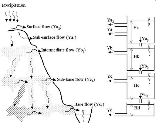
Brief Description of Tank Model
Figure 1 shows the Standard Tank Model and hypothetical water regimes in a watershed. This model is constructed of four vertical reservoirs, of which from top to bottom parts represents the Surface Reservoir (A), Intermediate Reservoir (B), Sub-base Reservoir (C), and Base Reservoir (D). In this concept, water can fill the underneath reservoir, and can go reversibly if evapotranspiration is so predominant. The horizontal outlet reflects the outflow, consisting of Surface Flow (Ya2), Subsurface Flow (Ya1), Intermediate Flow (Yb1), Sub-base Flow (Yc1),
and Base Flow (Yd1). Each outflow only occurs when the water level at each reservoir (Ha,
Hb, Hc and Hd) is higher than its outlet (Ha1, Ha2, Hb1 and Hc1). The outflow at each outlet is
also influenced by the characteristics of the outlet, i.e., A0, A1, A2, B0, B1, C0, C1, and D1, which further are called as the parameters of the Tank Model to be determined. All in all there are 12 (twelve) parameters.
Globally, the water balance equation can be written as follows:
3
Where, H is water level (mm), P is precipitation (mm/day), ET is evapotranspiration (mm/day), Y is total flow (mm/day), and t is time (day).
The total flow is the summation of the flow components that can be written as follows: )
The water balance in each reservoir in more detail can be written as:
)
Where, Ya, Yb, Yc and Yd are the horizontal flow components from each reservoir, and Ya0, Yb0 and Yc0 are the vertical components.
Practically, the total outflow (y) is frequently considered as the accumulation of the outflows from a system of water region. In a watershed, the total outflow can represent a river
discharge, and in a paddy field can be considered as drainage flow. In reality, it is very difficult or may be impossible to find out or distinguish the other outflows. It is clear that Tank Model only represent the study area globally. Commonly, the total outflow is the target to check out the workability of a Tank Model. Observation focused on the maximum values of the total outflow (Y) is needed in the study of flood. Meanwhile, information about minimum values or Base Flow (Yd1) will be useful for the water utilization planning, such as irrigation, fishery and so on, particularly during the dry periods. Thus, focus of observation might also be important in the determination of optimized parameters.
Optimization Technique
It is of interest to design an optimization technique capable of facilitating each structure of the Tank Model. Such optimization technique must not require detail information in every Tank Model. Herewith, the Tank Model is assumed as one Black Box and its behavior is observable when receiving updated parameters. We applied Marquardt algorithm, which in a simple case it is very quick and effective in finding the optimum parameter even for extremely non-linear equations (Marquardt, 1963; Setiawan and Shiozawa, 1992). Aside from that, it also has been equipped with maximum and minimum values for each parameter. Considering the basic structure of a Tank Model, the algorithm is reconstructed so it can receive the data of total outflow and calculation results from the model. With the Tank Model having 4 (four)
2) It has an input argument for receiving net of rainfall data minus evapotranspiration (X); and;
3) It has an output argument for transferring the calculation outflow of the Tank Model (Yc).
Herewith, in Pascal language, the procedure can be written as follows:
procedure TankModel(B:ArrayM; X:single; var Yc:single); begin
… end;
The complete writing of the program can be seen in Appendix 1. Inside this procedure, embodied (4) four procedure,each is used for calculating outflow from every reservoir. And, in the main program, the water level at each reservoir is calculated.
The Marquardt1 algorithm is constructed with the following considerations:
1) It has an input argument for receiving Minimum Value (Bmin) and Maximum Value (Bmax) parameters;
2) It has an input argument for receiving net of rainfall and evapotranspiration (X); 3) It has an input argument for receiving debit data (Yd); and
4) It has an input/output argument for receiving and transferring parameter (B).
Herewith, the designed procedure Marquardt is written as:
procedure Marquardt (Bmin,Bmax:ArrayM; X,Yd:ArrayN; var B:ArrayM); begin {Main of Marquardt}
…
end;{End of Marquardt}
The procedure Marquardt consists of procedure derivative with the function to carry out first derivation of the Tank Model numerically, procedure least square for minimizing error, and procedure gauss for the calculation of the renewed parameters.
By giving initial approximation of the parameters, iteration process continued until the sum of absolute changes of updated parameters reached a tolerable value, good conformity and less discrepancy of water balance. The last updated parameters then are considered as the final solutions.
Materials and Method
1
5
Here, the Optimization Technique was tested todetermine the parameters of the Standard Tank Model in 2 (two) watersheds, i.e., Terauchi Watershed (5055 ha) in Fukuoka, Japan, and Ciriung Watershed (120 ha) in Banten Province, Indonesia. From the Terauchi Watershed, daily data of rainfall, evapotranspiration, and water discharge were well recorded for 10 (ten) years, from 1986 through 1995 (Fukuda and Nakano, 2001). And, daily data from Ciriung Watershed were collected in 2002/2003 (Suprayogi, 2003).
To start the optimization process, we used initial values of parameters introduced by Sugawara et.al. (1986), such as seen in Table 1. The table also shows
the suggested Minimum Value and Maximum Value of each parameter. It was also necessary to give initial values of water level (Ha, Hb, Hc dan Hd) in each reservoir. Actually, the values were somewhat difficult to determine and even impossible to obtain from the field. Therefore, initial approximation was then done before the iteration process by giving a value of Hd=Yd/D1, i.e., when the Base Flow was at the lowest while other flow components were
assumed zero (i.e., during the dry season). Subsequently, calculation was done to produce new estimations for all water level values (Ha, Hb, Hc dan Hd) by checking out the water balance in the first year. If the water balance was good enough (minimum discrepancy), the water level value obtained was used as the initial condition to start the optimization process.
Updating all parameter values for each iteration was done was terminated after the absolute total of the changes in all parameters was less than the given tolerance value, i.e., 0.00001. The successfulness of the optimization technique was shown using coefficient of correlation (R) and 7 (seven) error indicators, i.e., 1) Root Mean Square Error (RMSE), 2) Mean Absolute Error (MAE), 3) Logarithmic RMSE (LOG), 4) Standard χ, 5) Squared Standard χ2; 6)
Relative Error (RE), and 7) Squared Relative Error (RR), which are written as the following equations (Fujihara, et.al., 2001):
Table 1. Initial Parameters
Parameter Initial Min Max
∑
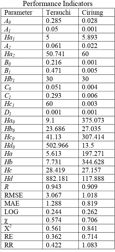
Results and Discussion
Table 2 shows the optimum parameter and error indicator after going through optimization process for both watersheds, i.e., Terauchi and Ciriung. At both watersheds, the Standard Tank Model resulted in very good water balance where the occurred discrepancy approaching zero. As such, the coefficient of correlation (R) was over 0.9, whilst the other error
indicator was almost less than one except for RMSE
which was over 3 and 1, repectively.
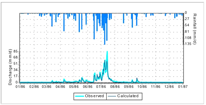
Hydrographic for Terauchi River in 1996 can be seen in Figure 2. The Standard Tank Model seems
successful in calculating low discharges but less successful in approaching the maximum descharges. Similar phenomenon was also shown in the
hydrographic for the previous years up to 1995. Here,
RMSE is always higher to others. Even as seen in Figure 3, the RMSE in 1991 reaches 8. Nevertheless,
almost all errors in that year were actually enlarging as compared to those in the previous and following years.
Figure 4 shows the hydrographic for Ciriung River. Different from Terauchi River, Ciriung River in the early year shows somewhat high discharges. But in the middle of the year starting from the end of June up to the early December of 2002 (dry season), it shows a decreasing discharges. Here, the Standard Tank Model seems to be successful in approaching the peak
discharges as compared to its nearness to the low discharges. Almost all of the error indicators are under one such as shown in Figure 5.
Table 2. Optimum Parameters and Performance Indicators
Parameter Terauchi Ciriung
A0 0.285 0.028
RMSE 3.067 1.018
7
Ob s e rve d C a lcula te d
01/87 12/86 11/86 10/86 09/86 08/86 07/86 06/86 05/86 04/86 03/86 02/86 01/86
D
is
c
h
ar
ge (
m
m
/d)85
68 51 34 17 0
R
a
in
fa
ll (
mm/
d
)
135 108 81 54 27 0
Figure 2. Hydrograph for Terauchi Watershed in 1996
Ob s e rved C a lcula te d
03/03 02/03 01/03 12/02 11/02 10/02 09/02 08/02 07/02 06/02 05/02 04/02 03/02
D
is
c
h
a
rg
e
(m
m
/d
)
8 6 4 2 0
R
a
in
fa
ll (
m
m
/d
)
65 52 39 26 13 0
Figure 4. Hydrograph for Ciriung Watershed in 2002/2003
9
This optimization process ran very fast in coming to convergence, i.e., it took time only in seconds. The number of iteration was seldom exceeding 100 times. It is possible in this process to set one or more parameters with known values to be constant. Eye fitting was also possibly done in the process in order to make the calculation more approaching to peak discharges or on the other way. This could be successfully done however with the compensation on decreasing the coefficient of correlation and effecting error indicators.This optimization technique has been made in the form of application package program2 in Window environment, using Delphi programming language (Appendix 2). Basically this program receives inputs of date, rainfall, potential evapotranspiration, and river discharges in mm/day unit. The outputs can be saved in the form of ASCII file for all parameters, water balance, intercept, slope, coefficient of correlation, error indicator including all water flow components (Y, Ya, Yb, Yc dan Yd). The hydrographic and regression curves can be saved in JPG file. The initial value of D1 could be given directly after data loading, and the process of
CHECK would result in the initial values for water level at each reservoir. If the initial values had given reasonable water balance, then OPTIMIZE could be run in order to update
parameters. Subsequently, the optimization process could be started and optimum parameter could be immediately obtained. Although this application is still limited for Standard Tank Model, yet this technique could be easily developed further to accommodate other type of Tank Model.
Conclusions
This paper has discussed parameter optimization technique for Standard Tank Model and here was tested for 2 (two) watersheds in Indonesia and Japan. This optimization technique is also equipped with the procedure for estimating the initial water level in each reservoir before starting the optimization process. The optimization process uses Marquardt algorithm showing its effectiveness and speed to determine the parameters. The test results of the two watersheds showed that the Standard Tank Model could represent the relation between rainfall minus potential evapotranspiration and water debit, which resulted in very good performance in terms of water balance, coefficient of correlation, and error indicators. This optimization technique has been made available in the form of application package program and readily developed for other Tank Models with different structures.
Acknowledgement
This research was a part of the JSPS-Core University Program in Applied Biosciences between The University of Tokyo and Institut Pertanian Bogor, 1998-2008.
References
2
Elhassan, A.M., A. Goto and M. Mizutani. 2001. Combining a tank model with a groundwater model for simulating regional groundwater flow in an alluvial fan. Transaction of
JSIDRE, 215:21-29.
Fujihara, Y., H. Tanakamaru, T. Hatta and A. Tada. 2001. Objective functions for calibration of rainfall-runoff models. In Proc. of Annual JSIDRE, 124-125, Morioka, 25-27 July. (In Japanese)
Fukuda, T. and Y. Nakano. 2001. Collections of hydrologic data for Terauchi Watershed. Irrigation and Water Utilization Laboratory, Kyushu University, Fukuoka. (Unpublished). Kadoya, M. and H. Tanakamaru. 1988. Flood run-off forecasting with long and short terms
run-off model. In Proc. of 6th Congress Asian and Pacific Regional Devision, International Association for Hydraulic Research, 624-631. Kyoto, 20-22 July.
Marquardt, D.W. 1963. An algorithm for least squares estimation of nonlinear parameters. J. Soc. Indust. Appl. Math, 11, 431-441.
Sugawara, M., I. Watanabe, E. Ozaki and Y. Katsuyama. 1986. Tank Model Programs for Personal Computer and the Way to Use. Research Report of National Research Center for Disaster Prevention, No37. Japan. (In Japanese).
Suprayogi, S. 2003. Study of Water Balance in Ciriung Sub-watershed, Cidanau Watershed. PhD diss., Stuty Program of Environment, Bogor Agricultural University, Bogor. (In Indonesian)
11
Appendix 1. Algorithm for Standard Tank Model in Pascal Language
procedure TankModel(B:ArrayM; Xi:single; var Yx:single);
var
YA0,YA1,YA2,YB0,YB1,YC0,YC1,YD1: single;
procedure TankA(Ha:real; B:ArrayM; var YA0,YA1,YA2:single); begin
YA0:=B[0]*Ha;
YA1:=B[1]*(Ha-B[2]); if YA1<0 then YA1:=0; YA2:=B[3]*(Ha-B[4]); if YA2<0 then YA2:=0; end;{TankA}
procedure TankB(Hb:real; B:ArrayM; var YB0,YB1:single); begin
YB0:=B[5]*Hb;
YB1:=B[6]*(Hb-B[7]); if YB1<0 then YB1:=0; end;{TankB}
procedure TankC(Hc:real; B:ArrayM; var YC0,YC1:single); begin
YC0:=B[8]*Hc;
YC1:=B[9]*(Hc-B[10]); if YC1<0 then YC1:=0; end;{TankC}
procedure TankD(Hd:real; B:ArrayM; var YD1:single); begin
YD1:=B[11]*Hd; end;{TankD}
begin {Main for TankModel}
Ha:=Ha+Xi;
TankA(Ha,B,YA0,YA1,YA2); Ha:=Ha-(YA0+YA1+YA2);
Hb:=Hb+YA0;
TankB(Hb,B,YB0,YB1); Hb:=Hb-(YB0+YB1);
Hc:=Hc+YB0;
TankC(Hc,B,YC0,YC1); Hc:=Hc-(YC0+YC1);
Yx:=YA1+YA2+YB1+YC1+YD1;
13
Appendix 2. Application Program for Optimization of Tank Model’s Parameters