Contemporary of Sciences
Physics, Chemistry and Mathematics
Editor: DENNIS LING
Contributing Authors: ANITA RAMLI BEH HOE GUAN
BALBIR SINGH MAHINDER SINGH CECILIA DEVI WILFRED
CHONG FAI KAIT HAMZAH SAKIDIN
HANITA DAUD HASNAH M ZAID HASSAN SOLEIMANI
LEE KEAN CHUAN LIM JUN WEI RADZUAN RAZALI TANG TOON BOON
Copyright c2015
PUBLISHED BYUTP PRESS
ISBN:XX-XXXX-XX
Licensed under the UTP Press, Universiti Teknologi PETRONAS (the “License”). You may not use this file except in compliance with the License. You may obtain a copy of the License from UTP Press, Universiti Teknologi PETRONAS. Unless required by applicable law or agreed to in writing, software distributed under the License is distributed on an “AS IS” BASIS,WITHOUT WARRANTIES OR CONDITIONS OF ANY KIND, either express or implied. See the License for the specific language governing permissions and limitations under the License.
Contents
I
Physics
1
Ferrite-CNT-Polymer Composite . . . 111.1 Introduction 11 1.2 Experimental 13 1.2.1 Materials . . . 13
1.2.2 Ferrite pereparation . . . 13
1.2.3 Composite preparation . . . 13
1.2.4 Characterization . . . 14
1.3 Results and discussion 14 1.3.1 Microstructural and morphological analysis . . . 14
1.3.2 Magnetic properties . . . 14
1.3.3 Electromagnetic wave absorbing properties . . . 16
1.4 Conclusion 18 1.5 References 19
2
Application in Enhanced Oil Recovery . . . 212.1 Introduction 21 2.2 Methodology 22 2.3 Results and discussion 22 2.3.1 Sample XRD . . . 22
2.3.2 Viscosity and IFT Test . . . 23
2.4 Conclusion 24
8.4 Results and discussion 91 12.3.4 Sum of Error Calculation For hydrostatic Neill Mapping Function, NMF(h) . . . 127
12.4 Conclusion 128
13
External Power Source for RFID Tags . . . 13113.1 Introduction 131
13.2 Thermoelectric Generator (TEG) Module 133
13.3 Methodology 134
13.3.1 Inductor Coil Transformer . . . 134 13.3.2 Circuit Design . . . 134
13.4 Results and discussion 135
13.5 Conclusion 138
13.6 References 139
14
Biodegradation . . . 14114.1 Introduction 141
14.2 Mathematical Model 141
14.3 Results and discussion 143
14.4 Conclusion 143
12. Global Positioning System (GPS)
NEILL’S MAPPING FUNCTION SIMPLIFICATION FOR DRY COMPONENT USING REGRESSION METHODS
The modeling of the GPS tropospheric delay mapping function should be revised by simplifying its mathematical model. The current tropospheric delay models use mapping functions in the form of continued fractions. This model is quite complex and need to be simplified. By using regression method, the dry (hydrostatics) mapping function models has been selected to be simplified. There are twenty six operations for dry mapping function component of Neill Mapping Function (NMF), to be carried out before getting the mapping function scale factor. So, there is a need to simplify the mapping function models to allow faster calculation and also better understanding of the models.
12.1 Introduction
The issue of atmospheric delay of Global Positioning system (GPS) signal is now extensively investigated to minimize the positioning error due to atmospheric delay, especially tropospheric and ionospheric delay (Sakidin, 2012a). The refraction index is a function of the actual tropospheric path through which the ray passes. The ray’s path begins at the receiver antenna ending at the last point of the effective troposphere. Tropospheric delay refers to the refraction of the GPS signal as it passes through the neutral atmosphere from the satellite to the earth. The effect causes the distance traveled by the signal to be longer than the actual geometric distance between the satellite and receiver. Hence, there is a need to introduce the simpler mathematical modeling of the mapping function model to increase the understanding of the model (Leick, 1995).
124 Chapter 12. Global Positioning System (GPS)
12.2 Tropospheric Delay
The tropospheric delay is measured in distance, and a typical zenith tropospheric delay would be between 2.3m to 2.5m (Misra & Enge, 2001), meaning that the troposphere causes a GPS range observation to have an apparent additional 2.5m distance between the ground based receiver and a satellite at zenith. The delay caused by the troposphere can be separated into two main components such as the hydrostatic delay and the wet delay (Saastamoinen, 1972). The hydrostatic delay is caused by the dry part of gases in the atmosphere, while the wet delay is caused solely by highly varying water vapor in the atmosphere. The hydrostatic delay makes up approximately 90% of the total tropospheric delay. The hydrostatic delay is entirely dependent on the atmospheric weather characteristics found in the troposphere. The hydrostatic delay in the zenith direction is typically about 2.3m (Businger et al., 1996 & Dodson et al., 1996).
Tropospheric delay can be reduced by using smaller mapping function. As a coefficient to the zenith tropospheric delay for both dry and also wet components, the value of mapping function can affect the total tropospheric delay. Mapping function depends on the elevation angle and produce larger value of mapping function by decreasing the elevation angle, especially for the elevation angles less than 5 degree (Sakidin & Chuan, 2012b). There is a need to minimize the mapping function in order to improve the total tropospheric delay for GPS signal. Saastamoinen model (1972) is selected for tropospheric delay calculation due to its accuracy about 3cm in zenith and this model is widely used for high accuracy GPS positioning (Mendes, 1999).
12.3 Mapping Function
12.3.1 Mapping Function Model Description
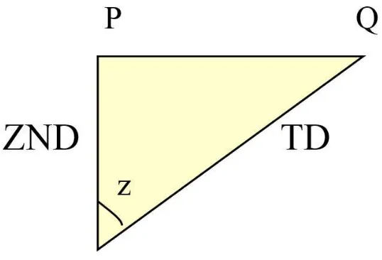
The tropospheric delay is the shortest in zenith direction and will become larger with increasing zenith angle. Projection of zenith path delays into slant direction is performed by application of a mapping function or obliquity factor, is defined as (Schuler, 2001):
m(z) = SND ZND=
T D
ZND (12.1)
where,
SND: slant neutral delay or total tropospheric delay (TD),
ZND: zenith neutral delay (total zenith delay). Referring to Figure 12.1, the tropospheric delay is shortest in zenith direction when the satellite at P and will become larger with increasing zenith angle at Q.
Unfortunately, this secant model is only an approximation assuming a planar surface of the earth and not taking the curvature of the earth into account. Moreover, the temperature and water vapor distribution may cause deviations from this simple formula. It can only be used for small zenith angle, from 0◦to 60◦(Saastamoinen, 1972). TD (total tropospheric delay) can be separated into two components such as a hydrostatic component (zenith hydrostatic delay, ZHD) and a wet component (zenith wet delay, ZWD) with their mapping function, m(z) as given below:
12.3 Mapping Function 125
Figure 12.1: Obliquity factor (mapping function) between zenith and slant direction (Sakidin and Chuan, 2012c).
In some cases, the mapping functions for wet and hydrostatic components are different. This representation allows the use of separate mapping functions for the hydrostatic and wet delay components (Schuler, 2001):
T D=ZHDmh(ε) +ZW Dmw(ε) (12.5)
where, ZHD : zenith hydrostatic delay (m) ZWD : zenith wet delay (m)mh(ε): the hydrostatic mapping function (no unit)mw(ε): the wet mapping function (no unit)
Nowadays, many modern mapping functions such asU NBabc,U NBab, Neill and some others have been established in a form of continued fraction, which introduce many operations. The number of operations for those mapping function models should be reduced from continued fraction form into simpler form to allow shorter computing time and better understanding of the models, but at the same time can give similar value for the mapping function scale factor (Sakidin, Ahmad & Bugis, 2014a).
12.3.2 Neill Mapping Function (NMF, 1996)
Neill (1996) proposed the new mapping function (NMF) based on temporal changes and geographic location rather than on surface meteorological parameters. He argued that all previously available mapping functions have been limited in their accuracy by the dependence on surface temperature, which causes three dilemmas. All of these are because there is more variability in temperature in the atmospheric boundary layer, from the Earth’s surface up to 2000 m. First, diurnal alterations in surface temperature cause much smaller variations than those calculated from the mapping functions. Second, seasonal changes in surface temperature are normally larger than upper atmosphere changes (but the computed mapping function yields artificially large seasonal variations). Third, the computed mapping function for cold summer days may not significantly differ from warm winter days. For example, actual mapping functions are quite different than computed values because of the difference in lapse rates and heights of the troposphere.
126 Chapter 12. Global Positioning System (GPS)
and applicability of the mapping functions . Through the least-square fit of four different latitude data sets, Niell (1996) showed that the temporal variation of the hydrostatic mapping function is sinusoidal within the scatter of the data.
The mapping functions derived by Arthur Neill in 1996, are the most widely used, and are known to be the most accurate and easily-implemented functions (Ahn, 2005). Neill Mapping Function hydrostatics component given in equation (12.6) below,
where,ε: elevation anglemh: hydrostatics mapping function H: station height above sea level (km).
For the hydrostaticsNMF mapping function, the parameterahat tabular latitudeϕi at time t from January 0.0 (in UT days) is given as:
ah(ϕ,t) =aavg(ϕ) +aamp(ϕ)cos
where DOY (day of year) is the adopted phase, DOY = 28 for Northern hemisphere and DOY = 211 for Southern hemisphere. The linear interpolation between the nearestah(ϕ,t)is used to obtain the value of parameterah(ϕ,t)which is stated as parameterahin equation (12.6). For parametersbh andch, the same procedure can be applied. Height correction coefficients are given asaht,bht and chtwere determined by a least-squares fit to the height correction at nine elevation angles (Neill, 1996).
Mendes (1999) analyzed the large number of mapping functions by comparing against ra-diosonde profiles from 50 stations distributed worldwide (32,467 benchmark values). The models that meet the high standards of modern space geodetic data analysis are Ifadis (1993), Lanyi (1984), Herring (1992), and Neill (1994). He found that for elevation angle above 15 degrees, the models Lanyi (1984), Herring (1992), and Neill (1994) yield identical mean biases and the best total error performance. At lower elevation angles, Ifadis (1993) and Neill (1994) are superior.
12.3.3 Simplification of hydrostatic Neill mapping function, NMF(h)
Regression method is used to find the same type of graph for the original NMF. However there is a slight difference for some points of the graph. From the statistical analysis, the difference between the original and the simplified model is small and not significant as described below.
NMF(h) model has been named as Y, while the simplified models have been named as Y1, Y2 and Y3. These four mapping function models give a graph of parabolic shape. However there is a slight difference between the Y model and the simplified models.
The simplified models (Y1, Y2 and Y3) have been generated using regression method, which give the model in a form of (Sakidin and Chuan, 2012b).
Y1=AXB (12.8)
whereY1: simplified NMF(h),A,B: constant,X : elevation angle (independent variable).
12.3 Mapping Function 127
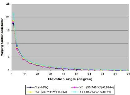
Figure 12.2: Graph of NMF(h) mapping function by regression.
12.3.4 Sum of Error Calculation For hydrostatic Neill Mapping Function, NMF(h)
Sum of error method can be used to show how the simplified models deviate from the original model. The smaller deviation is better, which shows that the simplified model is closer to the original model.
From the Table 3.1 above, although the sum of error is small (1.76), the Y1 model has not been selected due to it does not meet the constraint requirement (0.86), which is at 90 degree the mapping function scale factor should be unity. That is the constraint used in finding the mapping function model. Although the Y3 model meets the requirements, whereby the model gives big value of sum of error (14.21), which is most of the points are scattered quite far from the original NMF(h) mapping function model.
So, Y2 = 33.748X−0.782model has been selected as the simplification mapping function model for NMF(h) due the smallest sum of error (1.94) compared to the others and it’s mapping function gives unity at 90 degree elevation angle as given in Figure 12.2 below.
Table 12.1: Reduction percentage of model operation.
Model Number of operations Number of operations Reduction %Reduction
(Current method) (Regression method)
128 Chapter 12. Global Positioning System (GPS)
12.4 Conclusion
12.5 References 129
12.5 References
[1] Landt, J. (2005). The History of RFID. Potentials IEEE, 24(4), 8-11.
[2] Hosaka, R. (2007). An analysis for specifications of medical use RFID system as a wireless communication. Engineering in Medicine and Biology Society, 2007. EMBS 2007, 29th Annual International Conference of the IEEE, vol., no., pp. 2795-2798.
[3] Meng, Q., Jin, J. (2011). Design of low power active RFID tag in UHF band. Control, Automa-tion and Systems Engineering (CASE), pp.1-4, pp. 30-31.
[4] Nakao, S., Norimatsu, T., Yamazoe, T., Oshima, T., Watanabe, K., Minatozaki, K., Kobayashi, K. (2011). UHF RFID mobile reader for passive and active-tag communication, radio and wireless symposium (RWS). IEEE Conferences, 311-314.
[5] V. Daniel Hunt, Albert Puglia, Mike Puglia. 2007. A Guide to Radio Frequency Identification, USA. Wiley Publication.
[6] Harold G. Clampitt. 3rd edition 2007. The RFID Certification. Wiley Publication. [7] Steven Shepard. 2005. Radio Frequency Identification. USA. McGraw Hill Publication. [8] Dennis E. Brown. (2007). RFID Implementation, USA. Mc Graw Hill Publication.
[9]Bhattacharya, M., Chu, C.H., Mullen, T. (2008). A Comparative Analysis of RFID Adoption in Retail and Manufacturing Sectors. IEEE International Conference, 241-249.
[10]Watanabe, S. (2001). Wrist watch having thermoelectric generator (U.S 6304520 B1)
[11]Jeffrey, G., Caillat, T. (2003). Using the compatibility factor to design high efficiency seg-mented thermoelectric generators. MRS Proceedings, 793, S2.1.
[12]Jones, A., Hoare, R., Dontharaju, S., Tung, S., Sprang, R., Fazekas, J., Chain, J., Mickle, M. (2007). An automated, FPGA-based reconfigurable, low-power RFID tag. Microprocessors and Microsystems, 116-134.
[13]Tiliute, D. E. (2007). Battery management in wireless sensor networks. Electronics and Electrical Engineering, Kaunas Technology, 9-12.
[14]Damaschke, J. M. Design of a low input voltage converter for thermoelectric generator. IEEE Transaction on Industry Applications, 1203-1207.
130
Cha
pter
12.
Global
P
ositioning
System
(GPS)
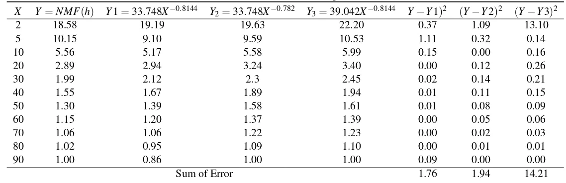
Table 12.2: Sum of error for NMF(h), Y and simplified models (Y1,Y2,Y3).
X Y =NMF(h) Y1=33.748X−0.8144 Y2=33.748X−0.782 Y3=39.042X−0.8144 Y−Y1)2 (Y−Y2)2 (Y−Y3)2
2 18.58 19.19 19.63 22.20 0.37 1.09 13.10
5 10.15 9.10 9.59 10.53 1.11 0.32 0.14
10 5.56 5.17 5.58 5.99 0.15 0.00 0.16
20 2.89 2.94 3.24 3.40 0.00 0.12 0.26
30 1.99 2.12 2.3 2.45 0.02 0.14 0.21
40 1.55 1.67 1.89 1.94 0.01 0.11 0.15
50 1.30 1.39 1.58 1.61 0.01 0.08 0.09
60 1.15 1.20 1.37 1.39 0.00 0.05 0.06
70 1.06 1.06 1.22 1.23 0.00 0.02 0.03
80 1.02 0.95 1.09 1.10 0.00 0.01 0.01
90 1.00 0.86 1.00 1.00 0.09 0.00 0.00